Tactics Reference
Robin Milner’s LCF system introduced a radical idea in the 1970s: let users extend the theorem prover with custom proof procedures, but channel all proof construction through a small trusted kernel. You could write arbitrarily clever automation, and if it produced a proof, that proof was guaranteed valid. Tactics are this idea fully realized. They are programs that build proofs, metaprograms that manipulate the proof state, search procedures that explore the space of possible arguments. When you write simp and Lean simplifies your goal through dozens of rewrite steps, you are invoking a sophisticated algorithm. When you write omega and Lean discharges a linear arithmetic obligation, you are running a decision procedure. The proof terms these tactics construct may be enormous, but they are checked by the kernel, and the kernel is small enough to trust. Think of tactics as the code you write, and the kernel as the one colleague who actually reads your pull requests.
Table of Contents
The following covers every user-facing tactic in core Lean 4 and its standard library, plus the Mathlib tactics this book uses. Click on any tactic name to jump to its documentation and examples. Related tactics share an entry.
abel- Prove equalities in abelian groupsac_nf- Normalize up to associativity and commutativityac_rfl- Close equalities up to associativity and commutativityadmit- Synonym for sorryaesop- General automation tacticall_goals- Apply tactic to all current goalsand_intros- Split every nested conjunctionany_goals- Apply tactic to any applicable goalapply- Apply hypotheses or lemmas to solve goalsapply?- Search the library for a lemma to applyapply_assumption- Apply one hypothesisapply_fun- Apply function to both sides of equalityapply_mod_cast- apply with casts normalizedapply_rules- Apply a rule set repeatedlyas_aux_lemma- Store the proof as a separate lemmaassumption- Use hypothesis matching goalassumption_mod_cast- assumption with casts normalizedbound- Prove inequalities from structurebv_decide- Decide bit vector goals with a SAT solverbv_normalize- Bit vector preprocessing onlybv_omega- Bit vector arithmetic via omegaby_cases- Perform case splittingby_contra- Proof by contradictioncalc- Chain equations and inequalitiescase- Select a goal by tagcase'- Select a goal by tag without closing itcases- Case analysis on inductive typescbv- Reduce goals by call-by-value evaluationchange- Restate a goal or hypothesischoose- Extract choice function from forall-existsclassical- Enable classical reasoning in a proofclear- Remove hypotheses from the contextclear_value- Forget the value of a local definitioncongr- Prove equality using congruence rulesconstructor- Break down conjunctions, existentials, and iffcontradiction- Find contradictions in hypothesesconv- Targeted rewriting in specific partsconvert- Prove by showing goal equals type of expressiondecide- Run decision proceduresdecide_cbv- Decide by call-by-value evaluationdecide +kernel- Decide by kernel reductiondecreasing_tactic- Default termination proofdecreasing_trivial- Extensible termination finisherdecreasing_with- Termination cleanup, then your tacticdelta- Raw definitional unfoldingdone- Assert no goals remaindsimp- Simplify with definitional rewrites onlyeq_refl- exact rfl with fast pathserw- Rewrite up to definitional unfoldingexact- Provide an exact proof termexact?- Search the library for a closing lemmaexact_mod_cast- exact with casts normalizedexfalso- Prove anything from Falseexists- Provide witnesses, then try trivialexpose_names- Make inaccessible names referableext- Prove equality of functions extensionallyext1- Apply one extensionality lemmaextract_lets- Hoist lets into the contextfail_if_success- Succeed only if a tactic failsfalse_or_by_contra- Change the goal to Falsefield_simp- Simplify field expressionsfin_cases- Split finite type into casesfirst- Try tactics until one succeedsfocus- Limit tactics to first goalfun_cases- Case split following a function’s equationsfunext- Equality of functions pointwisefun_induction- Induction following a function’s recursiongcongr- Prove inequalities using congruencegeneralize- Replace expressions with variablesget_elem_tactic- Discharge indexing boundsgrind- Proof search using congruence closuregrind_linarith- Linear arithmetic via grindgrind_order- Order reasoning via grindgrobner- Polynomial equalities via Gröbner basesgroup- Prove equalities in groupsguard_expr- Assert two expressions are equalguard_hyp- Assert the type of a hypothesisguard_target- Assert the shape of the goalhave- Introduce new hypotheseshave'- have with underscores as goalshaveI- Inline a fact for instance searchhint- Get tactic suggestionsif- Split on a decidable conditionimpossible- Prove that the goal has no proofinduction- Perform inductive proofsinfer_instance- Close a goal by instance resolutioninjection- Use injectivity of constructorsinjections- Repeat injection on all hypothesesinterval_cases- Split bounded values into casesintro- Introduce assumptions from implications and quantifiersintros- Introduce all binders with inaccessible namesitauto- Intuitionistic propositional tautologiesiterate- Run a tactic exactly n timesleft- Choose left side of disjunctionlet- Local definition with visible valueletI- Inline a definition for instance searchlet rec- Local recursive definitionlet_to_have- Turn lets into haveslia- Linear integer arithmetic via grindlift- Lift variable to higher typelift_lets- Float lets outwardlinarith- Prove linear inequalitieslinear_combination- Prove from linear combinationsmassumption- Close with a stateful hypothesismatch- Case analysis by pattern matchingmcases- Destructure a stateful hypothesismclear- Drop a stateful hypothesismconstructor- Split a stateful conjunctionmdup- Duplicate a stateful hypothesismexact- Close with a stateful termmexfalso- Stateful proof by contradictionmexists- Supply a stateful witnessmframe- Separate pure stateful hypothesesmhave- Add a stateful hypothesismintro- Introduce stateful hypothesesmleave- Leave proof mode and unfold the logicmleft- Choose the left stateful disjunctmodule- Prove equalities in modulesmpure- Move a pure hypothesis out of the stateful contextmpure_intro- Turn a pure stateful goal into a plain goalmrefine- Build a stateful goal from a termmrename_i- Name an inaccessible stateful hypothesismreplace- Overwrite a stateful hypothesismrevert- Move a stateful hypothesis into the goalmright- Choose the right stateful disjunctmspec- Apply a Hoare triple specificationmspecialize- Apply a stateful implicationmspecialize_pure- Apply a pure lemma to stateful hypothesesmstart- Enter stateful proof modemstop- Leave proof mode, keep the goalmvcgen- Generate verification conditionsmvcgen_trivial- Discharge trivial verification conditionsnative_decide- Decide by compiled evaluationnext- Select the next goalnlinarith- Handle nonlinear inequalitiesnofun- Prove an implication from an empty typenomatch- Eliminate an empty hypothesisnoncomm_ring- Prove in non-commutative ringsnorm_cast- Simplify by moving casts outwardnorm_num- Simplify numerical expressionsnth_rw- Rewrite only the nth occurrenceobtain- Destructure existentials and structuresomega- Solve linear arithmetic over Nat and Intopen ... in- Scope a namespace to one tacticpick_goal- Move specific goal to frontpositivity- Prove positivity goalspush_cast- Push casts inwardpush Not- Push negations inwardqify- Shift to rationalsrcases- Case analysis with patternsrefine- Apply with holes to fill laterrefine'- Refine where every underscore is a goalrename- Rename hypotheses for clarityrename_i- Name inaccessible hypothesesrepeat- Apply tactic repeatedly until failsrepeat'- Repeat recursively on all goalsrepeat1'- Repeat recursively, at least oncereplace- Overwrite a hypothesis with a new onerevert- Move hypotheses back to the goalrfl- Prove by reflexivityrfl'- rfl without smart unfoldingright- Choose right side of disjunctionring- Prove equalities in commutative ringsrintro- Introduce and destructure in one steprotate_left- Cycle the goal listrotate_right- Cycle the goal list the other wayrun_tac- Run TacticM code inlinerw- Rewrite using equalitiesrw?- Search the library for a rewriterwa- Rewrite, then assumptionrw_mod_cast- rw with casts normalizedset_option ... in- Scope an option to one tacticshow- Restate the goal up to definitional equalityshow_term- Report the proof term a tactic builtsimp- Apply simplification lemmassimpa- Simplify goal and hypothesis, then matchsimp_all- Simplify everything including hypothesessimp_rw- Rewrite with simplification at each stepsimp_wf- Unfold well-founded relation goalsskip- Do nothingsmt- Discharge goals to external SMT solverssolve- First alternative that closes the goalsolve_by_elim- Search by applying hypothesessorry- Admit goal without proofspecialize- Instantiate hypothesis with specific argumentssplit- Handle if-then-else and pattern matchingsplit_ifs- Case on if-then-else expressionsstop- Sorry the rest of the proofsubst- Substitute variable with its valuesubst_eqs- Substitute equations until fixpointsubst_vars- Substitute every variable equationsuffices- Reduce the goal to an intermediate claimswap- Swap first two goalssymm- Swap symmetric relationssymm_saturate- Add symmetric versions of hypothesestauto- Prove logical tautologiestrace- Print a messagetrace_state- Print the current goalstrans- Split transitive relationstrivial- Prove simple goals automaticallytry?- Search for a proof and suggest the scripttry- Attempt tactic, continue if failsunfold- Unfold a definition by its equationsunhygienic- Disable name hygiene for one tacticuse- Provide witnesses for existential goalsvcgen- Alternative verification condition generatorwith_reducible- Run with reducible transparencywith_unfolding_all- Run unfolding everythingzify- Shift natural numbers to integers·- Focus on the first goal
Logical Connectives
intro
The intro tactic moves hypotheses from the goal into the local context. When your goal is ∀ x, P x or P → Q, using intro names the bound variable or assumption and makes it available for use in the proof.
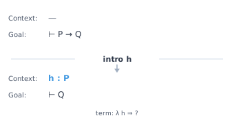
theorem intro_apply : ∀ x : Nat, x = x → x + 0 = x := by
  intro x h  -- Introduce x and hypothesis h : x = x
  simp       -- Simplify x + 0 = x
constructor
The constructor tactic applies the first constructor of an inductive type to the goal. For And (conjunction), it splits the goal into two subgoals. For Exists, it expects you to provide a witness. For Iff, it creates subgoals for both directions.
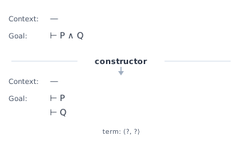
theorem constructor_example : True ∧ True := by
  constructor
  · trivial  -- Prove first True
  · trivial  -- Prove second True
left and right
The left and right tactics select which side of a disjunction to prove. When your goal is P ∨ Q, use left to commit to proving P or right to prove Q.
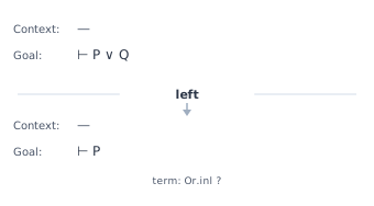
theorem or_example : 5 < 10 ∨ 10 < 5 := by
  left
  simp
use
The use tactic provides a concrete witness for an existential goal. When your goal is ∃ x, P x, using use t substitutes t for x and leaves you to prove P t.
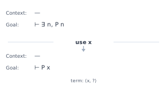
theorem use_example : ∃ x : Nat, x * 2 = 10 := by
  use 5  -- supply the witness; use tries rfl on what remains
obtain
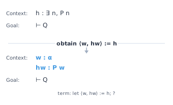
The obtain tactic extracts components from existential statements and structures in hypotheses. It combines have and pattern matching, letting you name both the witness and the proof simultaneously.
theorem have_example (x : Nat) : x + 0 = x := by
  have h : x + 0 = x := by simp
  exact h

theorem obtain_example (h : ∃ x : Nat, x > 5 ∧ x < 10) : ∃ y, y = 7 := by
  obtain ⟨_x, _hgt, _hlt⟩ := h  -- Destructure the existential
  exact ⟨7, rfl⟩
intros
The intros tactic introduces every leading binder at once with inaccessible names. Since you cannot refer to the names, it pairs with tactics that search the context such as assumption, or with rename_i to name them afterwards. In finished proofs prefer intro with explicit names.
theorem intros_example : ∀ (p q : Prop), p → q → p := by
  intros       -- introduce everything, with inaccessible names
  assumption   -- still usable by tactics that search the context
rintro
The rintro tactic combines intro with the destructuring patterns of rcases. A pattern like ⟨hp, hq⟩ introduces a conjunction and splits it in one step, and h | h splits a disjunction into two goals.
theorem rintro_example (p q : Prop) : p ∧ q → q ∧ p := by
  rintro ⟨hp, hq⟩  -- intro and destructure in one step
  exact ⟨hq, hp⟩
exists
The exists tactic provides witnesses for an existential goal and then runs trivial on whatever remains. It is the core Lean counterpart of Mathlib’s use, and for simple goals the two are interchangeable.
theorem exists_tactic_example : ∃ n : Nat, n > 3 := by
  exists 4  -- supplies the witness and tries trivial on the rest
and_intros
The and_intros tactic splits every nested conjunction in the goal into separate subgoals, where constructor would split only the outermost one.
theorem and_intros_example (p q r : Prop) (hp : p) (hq : q) (hr : r) : p ∧ q ∧ r := by
  and_intros <;> assumption  -- split every nested ∧ at once
nofun and nomatch
The nofun tactic proves a goal of the form P → Q when P is an empty type such as 1 = 2: the function it builds has no cases at all. The nomatch h tactic does the same with a hypothesis already in context, matching on h with zero alternatives.
theorem nofun_example : ¬ (1 = 2) := by
  nofun  -- a function with no cases: 1 = 2 has no constructors
theorem nomatch_example (h : False) : 1 = 2 := by
  nomatch h  -- match on h with no alternatives
Applying Lemmas
exact
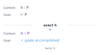
The exact tactic closes a goal by providing a term whose type matches the goal exactly. It performs no additional unification or elaboration beyond what is necessary.
theorem exact_example (h : 2 + 2 = 4) : 4 = 2 + 2 := by
  exact h.symm

/-- `refine` allows holes with ?_ -/
theorem refine_example : ∃ x : Nat, x > 5 := by
  refine ⟨10, ?_⟩  -- Use 10, but leave proof as a hole
  simp              -- Fill the hole: prove 10 > 5
apply
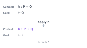
The apply tactic works backwards from the goal. Given a lemma h : A → B and a goal B, using apply h reduces the goal to proving A. It unifies the conclusion of the lemma with the current goal.
refine
The refine tactic is like exact but allows placeholders written as ?_ that become new goals. This lets you partially specify a proof term while deferring some parts.
theorem exact_example (h : 2 + 2 = 4) : 4 = 2 + 2 := by
  exact h.symm

/-- `refine` allows holes with ?_ -/
theorem refine_example : ∃ x : Nat, x > 5 := by
  refine ⟨10, ?_⟩  -- Use 10, but leave proof as a hole
  simp              -- Fill the hole: prove 10 > 5
convert
The convert tactic applies a term to the goal even when the types do not match exactly, generating side goals for the mismatches. It is useful when you have a lemma that is almost but not quite what you need.
theorem convert_example (x y : Nat) (h : x = y) : Nat.succ x = Nat.succ y := by
  convert rfl using 1
  rw [h]
specialize
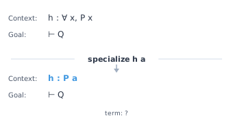
The specialize tactic instantiates a universally quantified hypothesis with concrete values, replacing the general statement with a specific instance in your context.
theorem specialize_example (h : ∀ x : Nat, x > 0 → x ≥ 1) : 5 ≥ 1 := by
  specialize h 5 (by simp)
  exact h
The refine' Variant
The refine' tactic is refine where plain underscores _ also become new goals instead of holes that must be filled by unification. It is the older behaviour, still useful when you want every missing argument to turn into a goal.
theorem refine_prime_example (p : Prop) (hp : p) : p ∧ True := by
  refine' ⟨hp, _⟩  -- plain underscores become new goals
  trivial
apply_rules
The apply_rules [r₁, r₂] tactic applies the listed lemmas and the local hypotheses repeatedly, depth first, until every goal is closed or the depth limit is reached. It is apply run as a search.
theorem apply_rules_example (p q r : Prop) (hp : p) (hq : q) (hr : r) : p ∧ q ∧ r := by
  apply_rules [And.intro]  -- apply the rule set repeatedly, then hypotheses
solve_by_elim and apply_assumption
The solve_by_elim tactic searches for a proof by repeatedly applying hypotheses from the local context, and apply_assumption performs one step of that search. Both are the engine that exact? and apply? hand over to once a candidate lemma is found.
theorem solve_by_elim_example (p q : Prop) (hp : p) (hpq : p → q) : q := by
  solve_by_elim  -- depth-first search using local hypotheses
theorem apply_assumption_example (p q : Prop) (hp : p) (hpq : p → q) : q := by
  apply_assumption  -- one step of that search: apply hpq
  exact hp
infer_instance
The infer_instance tactic closes a goal that is a type class instance by running instance resolution. It is the tactic form of the inferInstance term.
example : Inhabited Nat := by
  infer_instance  -- exact inferInstance
Context Manipulation
have
The have tactic introduces a new hypothesis into the context. You state what you want to prove as an intermediate step, prove it, and then it becomes available for the rest of the proof.
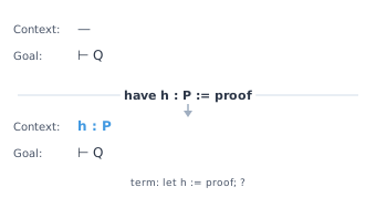
theorem have_example (x : Nat) : x + 0 = x := by
  have h : x + 0 = x := by simp
  exact h

theorem obtain_example (h : ∃ x : Nat, x > 5 ∧ x < 10) : ∃ y, y = 7 := by
  obtain ⟨_x, _hgt, _hlt⟩ := h  -- Destructure the existential
  exact ⟨7, rfl⟩
rename
The rename tactic changes the name of a hypothesis in the local context, making proofs more readable when auto-generated names are unclear.
theorem rename_example (h : 1 = 1) : 1 = 1 := by
  rename 1 = 1 => one_eq_one  -- rename the hypothesis by its type
  exact one_eq_one
revert
The revert tactic is the inverse of intro. It moves a hypothesis from the context back into the goal as an implication or universal quantifier, which is useful before applying induction or certain lemmas.
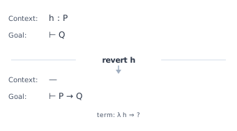
theorem revert_example (x : Nat) (h : x = 5) : x = 5 := by
  revert h x
  intro x h
  exact h
generalize
The generalize tactic replaces a specific expression in the goal with a fresh variable, abstracting over that value. This is useful when you need to perform induction on a compound expression.
theorem generalize_example : (2 + 3) * 4 = 20 := by
  generalize h : 2 + 3 = n  -- replace 2 + 3 by a fresh n with h : 2 + 3 = n
  omega
clear
The clear tactic removes hypotheses from the context. It fails if anything else still depends on them. Clearing noise before calling automation such as simp_all or grind can make those tactics both faster and more predictable.
set_option linter.unusedVariables false in
theorem clear_example (p q : Prop) (hp : p) (hq : q) : p := by
  clear hq  -- drop a hypothesis the proof does not need
  exact hp
clear_value
The clear_value x tactic turns a local definition x : α := v into an ordinary hypothesis x : α, forgetting the value. Record anything you need about the value first, as the example does with hx, or use the form clear_value (h : x = _) which adds that equation for you.
theorem clear_value_example : (let x := 5; x = 5) := by
  intro x
  -- x := 5 is a let binding; freeze it into an ordinary variable with a proof
  have hx : x = 5 := rfl
  clear_value x
  exact hx
rename_i
The rename_i tactic gives names to inaccessible hypotheses, the ones displayed with a dagger after intro without arguments or after cases. Names are assigned from the most recent hypothesis backwards.
theorem rename_i_example : ∀ n : Nat, n = n := by
  intro        -- introduces an inaccessible n✝
  rename_i m   -- give it a usable name
  exact rfl (a := m)
show and change
The show t tactic restates the goal as t, which must be definitionally equal to the current goal. It documents the proof and lets you unfold or fold definitions in place. The change t at h tactic does the same thing to a hypothesis.
theorem show_example (n : Nat) : n + 0 = n := by
  show n = n  -- restate the goal up to definitional unfolding
  rfl
theorem change_example (n : Nat) (h : n + 0 = 5) : n = 5 := by
  change n = 5 at h  -- the same, applied to a hypothesis
  exact h
suffices
The suffices h : p from e tactic is have run backwards: it proves the goal from p using e right away, and leaves p itself as the remaining goal. Use it when the reduction is obvious and the interesting work is proving the intermediate statement.
theorem suffices_example (p q : Prop) (hp : p) (hpq : p → q) : q := by
  suffices h : p from hpq h  -- reduce the goal to p
  exact hp
replace
The replace h := e tactic is have h := e followed by clearing the old h. It keeps the context tidy when a hypothesis is only ever used to derive a stronger one.
theorem replace_example (p q : Prop) (hp : p) (hpq : p → q) : q := by
  replace hp := hpq hp  -- hp : q now; the old hp is gone
  exact hp
have', haveI and letI
The have' tactic is have built on refine', so underscores in the value become new goals. The haveI and letI tactics add a fact or definition that is inlined into the proof term rather than bound with a let, which matters when the value is a type class instance that later elaboration must see. For propositions, plain have does the same job, and Mathlib’s linter will say so.
theorem have_prime_example (p : Prop) (hp : p) : p := by
  have' h := hp  -- have via refine', so _ makes goals
  exact h
example : Nat := by
  haveI : Inhabited Nat := ⟨0⟩  -- inlined, visible to instance search
  exact default
example : Nat := by
  letI : Inhabited Nat := ⟨0⟩   -- like haveI but keeps the value
  exact default
let and let rec
The let x := v tactic adds a local definition whose value stays visible to the goal, unlike have, which forgets it. The let rec tactic defines a local recursive function or lemma inside a proof, with the usual termination checking.
theorem let_example : 2 + 2 = 4 := by
  let x := 2       -- a local definition whose value stays visible
  show x + x = 4
  rfl
theorem let_rec_example : 10 ≤ 100 := by
  let rec go : ∀ n : Nat, n ≤ n + 90 := fun n => by omega
  exact go 10
extract_lets, lift_lets and let_to_have
These three tactics manage let bindings inside the goal. The extract_lets tactic moves them into the local context as definitions, lift_lets floats them outward so they can be introduced, and let_to_have converts bindings whose values are never used in the type into plain haves.
theorem extract_lets_example : (let x := 5; x + 1) = 6 := by
  extract_lets x   -- hoist the let into the context as x := 5
  rfl
theorem lift_lets_example : (let x := 5; x + 1) = 6 := by
  lift_lets        -- move lets outward in the goal
  intro x
  rfl
theorem let_to_have_example : (let x := 5; x + 1) = 6 := by
  let_to_have      -- turn lets whose value is not needed into haves
  rfl
expose_names
The expose_names tactic renames every inaccessible hypothesis to a fresh accessible name so a proof script can refer to it. It is what Try this suggestions insert when they need to mention such a variable. In hand-written proofs, naming things with intro or rename_i is clearer.
theorem expose_names_example : ∀ n : Nat, n = n := by
  intro
  expose_names  -- rename every inaccessible n✝ to something referable
  rfl
subst_vars and subst_eqs
The subst_vars tactic runs subst on every hypothesis of the form x = t or t = x where x is a local variable. The subst_eqs tactic repeatedly substitutes using the equations in the context, replacing left sides by right sides, until nothing changes.
theorem subst_vars_example (x : Nat) (h : x = 2) : x + x = 4 := by
  subst_vars  -- substitute every hypothesis of the form var = term
  rfl
theorem subst_eqs_example (a b : Nat) (h₁ : a = 1) (h₂ : b = a) : b = 1 := by
  subst_eqs
  rfl
symm_saturate
The symm_saturate tactic adds, for every hypothesis h : a ~ b whose relation has a @[symm] lemma, the flipped version h_symm : b ~ a. It is a cheap way to make assumption and simp succeed without stating the symmetric fact by hand.
theorem symm_saturate_example (a b : Nat) (h : a = b) : b = a := by
  symm_saturate  -- adds h_symm : b = a for every symmetric hypothesis
  assumption
Rewriting and Simplifying
rw (rewrite)
The rw tactic replaces occurrences of the left-hand side of an equality with the right-hand side. Use rw [←h] to rewrite in the reverse direction. Multiple rewrites can be chained in a single rw [h1, h2, h3].
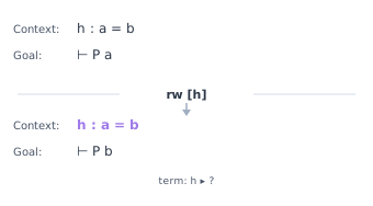
theorem rw_example (a b : Nat) (h : a = b) : a + 2 = b + 2 := by
  rw [h]  -- Rewrite a to b using h

theorem simp_example (x : Nat) : x + 0 = x ∧ 0 + x = x := by
  simp  -- Simplifies both sides
Tip
rwuses the first matching occurrence to instantiate the rewrite rule, then rewrites matching occurrences of that instantiated expression; it can rewrite more than one occurrence. Userw [h] at hypto rewrite in a hypothesis instead of the goal. If rewriting fails due to dependent types or metavariables, trysimp_rwwhich handles these cases more gracefully. Usenth_rw n [h]to target a specific occurrence.
simp
The simp tactic repeatedly applies lemmas marked with @[simp] to simplify the goal. It handles common algebraic identities, list operations, and logical simplifications automatically.
theorem rw_example (a b : Nat) (h : a = b) : a + 2 = b + 2 := by
  rw [h]  -- Rewrite a to b using h

theorem simp_example (x : Nat) : x + 0 = x ∧ 0 + x = x := by
  simp  -- Simplifies both sides
Tip
Use
simp only [lemma1, lemma2]for reproducible proofs. Baresimpcan break when new simp lemmas are added to the library. Usesimp?to see which lemmas were applied, then replace withsimp only [...]for stability. In Mathlib code reviews, baresimpat non-terminal positions is discouraged.
simp_all
The simp_all tactic simplifies both the goal and all hypotheses simultaneously, using each simplified hypothesis to help simplify the others.
theorem simp_all_example (x : Nat) (h : x = 0) : x + x = 0 := by
  simp_all
simp_rw
The simp_rw tactic rewrites using the given lemmas but applies simplification at each step, which helps when rewrites would otherwise fail due to associativity or other issues.
theorem simp_rw_example (x y : Nat) : (x + y) + (y + x) = 2 * (x + y) := by
  simp_rw [Nat.add_comm y x]
  ring
nth_rw
The nth_rw tactic rewrites only a specific occurrence of a pattern, counting from 1. This gives precise control when an expression appears multiple times and you only want to change one instance.
theorem nth_rewrite_example (x : Nat) : x + x + x = 3 * x := by
  nth_rw 2 [← Nat.add_zero x]  -- Rewrite only the second occurrence of x
  simp
  ring
norm_num
The norm_num tactic evaluates and simplifies numeric expressions, proving goals like 2 + 2 = 4 or 7 < 10 by computation. It handles arithmetic in various number types.
theorem norm_num_example : 2 ^ 3 + 5 * 7 = 43 := by
  norm_num
norm_cast
The norm_cast tactic normalizes expressions involving type coercions by pushing casts outward and combining them, making goals about mixed numeric types easier to prove.
theorem norm_cast_example (n : Nat) : (n : Int) + 1 = ((n + 1) : Int) := by
  norm_cast
push_cast
The push_cast tactic pushes type coercions inward through operations, distributing a cast over addition, multiplication, and other operations.
set_option linter.unusedTactic false in
theorem push_cast_example (n m : Nat) : ((n + m) : Int) = (n : Int) + (m : Int) := by
  push_cast
  rfl
conv
The conv tactic enters a conversion mode that lets you navigate to specific subexpressions and rewrite only there. It is invaluable when rw affects the wrong occurrence or when you need surgical precision.
theorem conv_example (x y : Nat) : x + y = y + x := by
  conv =>
    lhs  -- Focus on left-hand side
    rw [Nat.add_comm]
Tip
Navigation commands in
convmode:lhs/rhsselect sides of an equation,arg nselects the nth argument,extintroduces binders, andenter [1, 2]navigates by path. Useconv_lhsorconv_rhsas shortcuts when you only need to work on one side of an equation.
rwa and erw
The rwa tactic is rw followed by assumption, for the common case where a rewrite turns the goal into one of the hypotheses. The erw tactic is rw that unfolds definitions while matching the rewrite pattern, so it finds instances that plain rw misses at the cost of sometimes rewriting more than you expected.
theorem rwa_example (a b : Nat) (h : a = b) : a + 0 = b := by
  rwa [Nat.add_zero]  -- rw, then assumption
theorem erw_example (a b : Nat) (h : a = b) : a + 0 = b := by
  erw [h, Nat.add_zero]  -- rw that unfolds definitions while matching
dsimp
The dsimp tactic is simp restricted to definitional rewrites: beta reduction, unfolding of reducible definitions, and lemmas proved by rfl. Because every step is definitional, the result is still definitionally equal to the original goal, which simp does not guarantee.
theorem dsimp_example (a : Nat) : (fun x => x + 0) a = a := by
  dsimp  -- only definitional rewrites, so the result is still rfl-equal
simpa
The simpa using h tactic simplifies both the goal and h with the same simp set and closes the goal when the two match. Without using, it simplifies the goal and finishes with assumption.
theorem simpa_example (a : Nat) (h : a = 0) : a + 0 = 0 := by
  simpa using h  -- simp the goal and h, then close by matching
unfold and delta
The unfold f tactic replaces f by its definition using the equation lemmas Lean generated for it, which handles pattern matching and recursion sensibly. The delta f tactic does raw definitional unfolding, exposing the compiled match and recursors. Use unfold, and reach for delta only when unfold cannot find an equation to apply.
def double (n : Nat) := 2 * n
theorem unfold_example : double 3 = 6 := by
  unfold double  -- replace by the equation lemma
  rfl
theorem delta_example : double 3 = 6 := by
  delta double   -- raw definitional unfolding, no equation lemmas
  rfl
exact_mod_cast and friends
The exact_mod_cast, apply_mod_cast, rw_mod_cast and assumption_mod_cast tactics are their namesakes with norm_cast run first on the goal and on the term or hypothesis involved. They let you use a lemma stated over Nat to close a goal stated over Int, or the other way around, without writing the cast lemmas yourself.
theorem exact_mod_cast_example (a b : Nat) (h : (a : Int) = b) : a = b := by
  exact_mod_cast h
theorem apply_mod_cast_example (a b : Nat) (h : (a : Int) = b) : a = b := by
  apply_mod_cast h
theorem rw_mod_cast_example (a b c : Nat) (h : b = c) : ((a + b : Nat) : Int) = a + c := by
  rw_mod_cast [h]  -- normalize casts, then rewrite with h
theorem assumption_mod_cast_example (a b : Nat) (h : (a : Int) = b) : a = b := by
  assumption_mod_cast
ac_rfl and ac_nf
The ac_rfl tactic closes an equality whose two sides are equal up to associativity and commutativity of operators that carry Std.Associative and Std.Commutative instances. The ac_nf tactic normalizes both sides into a canonical form instead of closing the goal, which is useful as a preprocessing step before rw.
theorem ac_rfl_example (a b c : Nat) : a + b + c = c + b + a := by
  ac_rfl  -- equal up to associativity and commutativity
theorem ac_nf_example (a b c : Nat) : a + b + c = c + (b + a) := by
  ac_nf   -- normalize both sides instead of closing outright
Reasoning with Relations
rfl (reflexivity)
The rfl tactic proves goals of the form a = a where both sides are definitionally equal. It works even when the equality is not syntactically obvious but follows from definitions.
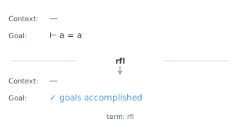
theorem rfl_example (x : Nat) : x = x := by
  rfl
symm
The symm tactic reverses a symmetric relation like equality. If your goal is a = b and you have h : b = a, using symm on h or the goal makes them match.
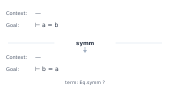
theorem symm_example (x y : Nat) (h : x = y) : y = x := by
  symm
  exact h
trans
The trans tactic splits a transitive goal like a = c into two subgoals a = b and b = c for a chosen intermediate value b. It works for any transitive relation.
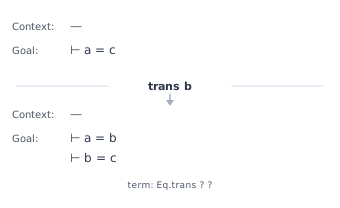
theorem trans_example (a b c : Nat) (h1 : a ≤ b) (h2 : b ≤ c) : a ≤ c := by
  trans b
  · exact h1
  · exact h2
subst
The subst tactic eliminates a variable by substituting it everywhere with an equal expression. Given h : x = e, using subst h replaces all occurrences of x with e and removes x from the context.
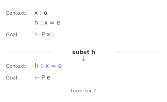
theorem subst_example (x y : Nat) (h : x = 5) : x + y = 5 + y := by
  subst h
  rfl
ext (extensionality)
The ext tactic proves equality of functions, sets, or structures by showing they agree on all inputs or components. It introduces the necessary variables and reduces the goal to pointwise equality.
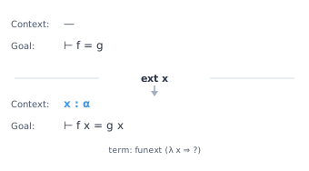
theorem ext_example (f g : Nat → Nat)
    (h : ∀ x, f x = g x) : f = g := by
  ext x
  exact h x
calc
The calc tactic provides a structured way to write chains of equalities or inequalities. Each step shows the current expression, the relation, and the justification, mirroring traditional mathematical proofs.
theorem calc_example (a b c : Nat)
    (h1 : a = b) (h2 : b = c) : a = c := by
  calc a = b := h1
       _ = c := h2
apply_fun
The apply_fun tactic applies a function to both sides of an equality hypothesis. It automatically generates a side goal requiring the function to be injective when needed.
theorem apply_fun_example (x y : Nat) (h : x = y) : x + 2 = y + 2 := by
  apply_fun (· + 2) at h
  exact h
congr
The congr tactic reduces an equality goal f a = f b to proving a = b, applying congruence recursively. It handles nested function applications by breaking them into component equalities.
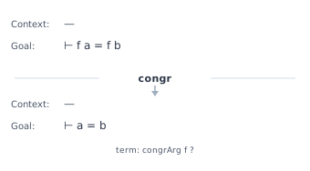
theorem congr_example (f : Nat → Nat) (x y : Nat) (h : x = y) : f x = f y := by
  congr
gcongr
The gcongr tactic proves inequalities by applying monotonicity lemmas. It automatically finds and applies lemmas showing that operations preserve ordering, such as adding to both sides of an inequality.
theorem gcongr_example (x y a b : Nat) (h1 : x ≤ y) (h2 : a ≤ b) : x + a ≤ y + b := by
  gcongr
linear_combination
The linear_combination tactic proves an equality by showing it follows from a linear combination of given hypotheses. You specify the coefficients, and it verifies the algebra.
theorem linear_combination_example (x y : ℚ) (h1 : 2*x + y = 4) (h2 : x + 2*y = 5) :
    x + y = 3 := by
  linear_combination (h1 + h2) / 3
positivity
The positivity tactic proves goals asserting that an expression is positive, nonnegative, or nonzero. It analyzes the structure of the expression and applies appropriate lemmas automatically.
set_option linter.unusedVariables false in
theorem positivity_example (x : ℚ) (h : 0 < x) : 0 < x^2 + x := by
  positivity
bound
The bound tactic proves inequality goals by recursively analyzing expression structure and applying bounding lemmas. It is particularly effective for expressions built from well-behaved operations.
theorem bound_example (x y : ℕ) : x ≤ x + y := by
  bound
eq_refl and rfl'
The eq_refl tactic is exact rfl with a few fast paths, and rfl' is rfl with smart unfolding switched off, so it will unfold definitions that rfl leaves alone. Plain rfl is the right default; these are for the rare cases where it stops short.
theorem eq_refl_example : 2 + 2 = 4 := by
  eq_refl  -- exact rfl with a fast path
theorem rfl_prime_example : 2 + 2 = 4 := by
  rfl'     -- rfl with smart unfolding disabled
funext and ext1
The funext x tactic reduces an equality between functions to an equality between their values at an arbitrary x. The ext1 tactic applies exactly one extensionality lemma, where ext keeps applying them as far as it can.
theorem funext_example : (fun n : Nat => n + 0) = (fun n => n) := by
  funext n  -- reduce equality of functions to equality at n
  rfl
theorem ext1_example (a b : Nat × Nat) (h1 : a.1 = b.1) (h2 : a.2 = b.2) : a = b := by
  ext1 <;> assumption  -- apply exactly one extensionality lemma
Reasoning Techniques
cases
The cases tactic performs case analysis on an inductive type, creating separate subgoals for each constructor. For a natural number, it splits into the zero case and the successor case.
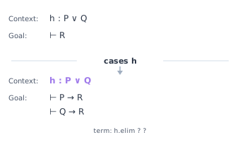
theorem cases_example (n : Nat) : n = 0 ∨ n > 0 := by
  cases n with
  | zero => left; rfl
  | succ _m => right; exact Nat.succ_pos _

theorem induction_example (n : Nat) : n + 0 = n := by
  induction n with
  | zero => rfl
  | succ n _ih => rfl
induction
The induction tactic sets up a proof by induction on an inductive type. It creates a base case for each non-recursive constructor and an inductive case with an induction hypothesis for each recursive constructor.
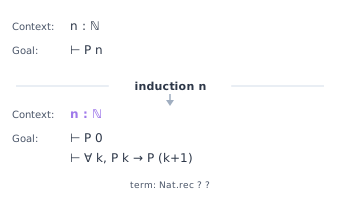
theorem cases_example (n : Nat) : n = 0 ∨ n > 0 := by
  cases n with
  | zero => left; rfl
  | succ _m => right; exact Nat.succ_pos _

theorem induction_example (n : Nat) : n + 0 = n := by
  induction n with
  | zero => rfl
  | succ n _ih => rfl
Tip
Use
induction n with | zero => ... | succ n ih => ...for structured case syntax. If your induction hypothesis is too weak, tryreverton additional variables before inducting, or useinduction n generalizing x yto strengthen the hypothesis. For mutual or nested induction, considerinduction ... usingwith a custom recursor.
split
The split tactic splits goals involving if-then-else expressions or pattern matching into separate cases. It creates subgoals for each branch with the appropriate condition as a hypothesis.
def abs (x : Int) : Nat :=
  if x ≥ 0 then x.natAbs else (-x).natAbs

theorem split_example (x : Int) : abs x ≥ 0 := by
  unfold abs
  split <;> simp
split_ifs
The split_ifs tactic finds all if-then-else expressions in the goal and splits on their conditions, creating cases for each combination of true and false branches.
theorem split_ifs_example (p : Prop) [Decidable p] (x y : Nat) :
    (if p then x else y) ≤ max x y := by
  split_ifs
  · exact le_max_left x y
  · exact le_max_right x y
contradiction
The contradiction tactic closes the goal by finding contradictory hypotheses in the context, such as h1 : P and h2 : ¬P, or an assumption of False.
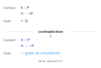
theorem contradiction_example (h1 : False) : 0 = 1 := by
  contradiction

theorem exfalso_example (h : 0 = 1) : 5 = 10 := by
  exfalso  -- Goal becomes False
  simp at h
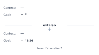
exfalso
The exfalso tactic changes any goal to False, applying the principle of explosion. Use this when you can derive a contradiction from your hypotheses.
theorem contradiction_example (h1 : False) : 0 = 1 := by
  contradiction

theorem exfalso_example (h : 0 = 1) : 5 = 10 := by
  exfalso  -- Goal becomes False
  simp at h
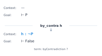
by_contra
The by_contra tactic starts a proof by contradiction. It adds the negation of the goal as a hypothesis and changes the goal to False, requiring you to derive a contradiction.
theorem by_contra_example (n : Nat) (h : ¬ n ≠ 0) : n = 0 := by
  by_contra hne  -- assume n ≠ 0 and derive False
  exact h hne
Proof of negation vs proof by contradiction: These are often confused but differ in an important way. A proof of negation proves ¬P by assuming P and deriving False. This is constructive since ¬P is defined as P → False. A proof by contradiction proves P by assuming ¬P and deriving False. This requires classical logic (double negation elimination) because you must go from ¬¬P to P. The by_contra tactic performs proof by contradiction and relies on Classical.byContradiction. If you are proving a negation, you can use intro h instead, which is constructive.
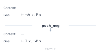
push Not
The push Not tactic pushes negations through quantifiers and connectives using De Morgan’s laws. It transforms ¬∀ x, P x into ∃ x, ¬P x and similar patterns.
-- `push Not` pushes negations inward through quantifiers and connectives
theorem push_neg_example : ¬(∀ x : Nat, ∃ y, x < y) ↔ ∃ x : Nat, ∀ y, ¬(x < y) := by
  push Not
  rfl
by_cases
The by_cases tactic splits the proof into two cases based on whether a proposition is true or false, adding the proposition as a hypothesis in one branch and its negation in the other.
theorem by_cases_example (p : Prop) : p ∨ ¬p := by
  by_cases h : p
  · left; exact h
  · right; exact h
choose
The choose tactic extracts a choice function from a hypothesis of the form ∀ x, ∃ y, P x y. It produces a function f and a proof that ∀ x, P x (f x).
theorem choose_example (h : ∀ x : Nat, ∃ y : Nat, x < y) :
    ∃ f : Nat → Nat, ∀ x, x < f x := by
  choose f hf using h
  exact ⟨f, hf⟩
lift
The lift tactic replaces a variable with one of a more specific type when you have a proof justifying the lift. For example, lifting an integer to a natural number given a proof it is nonnegative.
theorem lift_example (n : ℤ) (hn : 0 ≤ n) : ∃ m : ℕ, (m : ℤ) = n := by
  lift n to ℕ using hn
  exact ⟨n, rfl⟩
zify
The zify tactic converts a goal about natural numbers to one about integers, which often makes subtraction and other operations easier to handle since integers are closed under subtraction.
theorem zify_example (n m : ℕ) (_ : n ≥ m) : (n - m : ℤ) = n - m := by
  zify
qify
The qify tactic converts a goal about integers or naturals to one about rationals, enabling division and making certain algebraic manipulations possible.
theorem qify_example (a b : ℕ) (h : a ≤ b) : (a : ℚ) ≤ b := by
  qify at h  -- move the hypothesis into ℚ where the goal lives
  exact h
rcases
The rcases tactic is cases with patterns. ⟨a, b⟩ destructures a structure or conjunction, a | b splits a sum or disjunction, rfl substitutes an equation, and - discards a component. Patterns nest, so one line can take apart a hypothesis that would otherwise need several cases. The obtain tactic uses the same pattern language.
theorem rcases_example (p q r : Prop) (h : p ∧ (q ∨ r)) : (p ∧ q) ∨ (p ∧ r) := by
  rcases h with ⟨hp, hq | hr⟩  -- destructure nested ∧ and ∨ in one pattern
  · exact Or.inl ⟨hp, hq⟩
  · exact Or.inr ⟨hp, hr⟩
match
The match tactic performs case analysis with the same syntax as a match expression in a definition. Each alternative becomes a goal with the pattern variables in context. It is often clearer than cases when the patterns are nested or when you want to name the cases by shape.
theorem match_example (n : Nat) : n + 0 = n := by
  match n with
  | 0 => rfl
  | k + 1 => rfl
fun_induction and fun_cases
The fun_induction f x tactic performs induction following the recursive structure of the function f rather than the structure of its argument, producing one goal per equation of f with an induction hypothesis for each recursive call. The fun_cases tactic gives the same case split without the induction hypotheses. Both use the functional induction principle Lean generates for every recursive definition.
def half : Nat → Nat
  | 0 => 0
  | 1 => 0
  | n + 2 => half n + 1
theorem fun_induction_example (n : Nat) : half n ≤ n := by
  fun_induction half n <;> omega  -- one case per equation of half
theorem fun_cases_example (n : Nat) : half n ≤ n := by
  fun_cases half n   -- the same split, without induction hypotheses
  · simp
  · simp
  · simp
    exact fun_induction_example _ |>.trans (by omega)
injection and injections
The injection h tactic uses the fact that constructors are injective: from h : Nat.succ a = Nat.succ b it derives a = b. The injections tactic applies injection to every hypothesis repeatedly, which unpacks nested constructor equalities such as a :: b :: l = c :: d :: m. Both close the goal outright when the constructors differ.
theorem injection_example (a b : Nat) (h : a + 1 = b + 1) : a = b := by
  injection h  -- constructors are injective: succ a = succ b gives a = b
theorem injections_example (a b : Nat)
    (h : Nat.succ (Nat.succ a) = Nat.succ (Nat.succ b)) : a = b := by
  injections   -- repeat injection as far as it goes
if
The if h : c then t else e tactic splits the proof on a decidable condition, with h : c in one branch and h : ¬c in the other. It is by_cases with the branches written inline.
theorem if_example (n : Nat) : n = 0 ∨ n ≠ 0 := by
  if h : n = 0 then exact Or.inl h else exact Or.inr h
false_or_by_contra
The false_or_by_contra tactic changes the goal to False while keeping as much information as possible. It introduces the premise of an implication or negation, and for a plain proposition P it adds ¬P to the context. It is the preprocessing step that omega, grind and bv_decide run before their own reasoning.
theorem false_or_by_contra_example (p : Prop) (h : ¬¬p) : p := by
  false_or_by_contra  -- goal becomes False, with ¬p in context
  exact h (by assumption)
classical
The classical tactic makes the axiom of choice available for the rest of the proof so that every proposition is decidable and by_cases works on any statement. It is a scoping tactic: the instance it adds exists only within the current proof.
theorem classical_example (p : Prop) : p ∨ ¬p := by
  classical  -- make Classical.propDecidable available
  exact Classical.em p
Searching
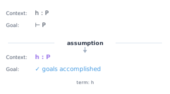
assumption
The assumption tactic closes the goal if there is a hypothesis in the context that exactly matches. It searches through all available hypotheses to find one with the right type.
theorem assumption_example (P Q : Prop) (h1 : P) (_h2 : Q) : P := by
  assumption  -- Finds h1
trivial
The trivial tactic tries a collection of simple tactics including rfl, assumption, and contradiction to close easy goals without you specifying which approach to use.
theorem trivial_example : True := by
  trivial
decide
The decide tactic evaluates decidable propositions by computation. For finite checks like 2 < 5 or membership in a finite list, it simply computes the answer and closes the goal.
theorem decide_example : 3 < 5 := by
  decide
Note
decideworks in the kernel and produces small proof terms but can be slow.native_decidecompiles the decision procedure to native code and runs it, which is much faster, but the kernel never sees the computation. Instead each call introduces a fresh axiom asserting the result, and#print axiomslists it by name (for examplebig._native.native_decide.ax_1_1). You are trusting the compiler and runtime for that one fact. For quick checks usedecide; for expensive computations like verifying grid states in our Game of Life proofs,native_decideis essential.
cbv
The cbv tactic reduces the goal by call-by-value evaluation: it unfolds definitions and evaluates arguments innermost-first, the same reduction strategy the compiler uses. It sits between simp and decide. Where simp rewrites with lemmas and decide demands a full Decidable instance, cbv just runs the computation. It accepts a location (cbv at h), a step limit (set_option cbv.maxSteps n), and short-circuits Or and And. Mark a definition @[cbv_opaque] to stop cbv from unfolding it, and tag an equation @[cbv_eval] to give cbv a rewrite rule to use in its place, which is how you keep an expensive or irrelevant definition folded while still computing around it. The companion decide_cbv finishes a decidable goal using the same evaluator, often succeeding where plain decide would be slow or stack-heavy.
-- `cbv` reduces the goal by call-by-value evaluation: it unfolds definitions
-- and evaluates arguments innermost-first, the same strategy the compiler uses.
theorem cbv_map : [1, 2, 3].map (· * 2) = [2, 4, 6] := by cbv

theorem cbv_fold : (List.range 5).foldl (· + ·) 0 = 10 := by cbv

-- `decide_cbv` finishes a decidable goal using call-by-value evaluation,
-- often succeeding where plain `decide` would be slow or stack-heavy.
theorem decide_cbv_example : (List.range 100).length = 100 := by decide_cbv

-- `@[cbv_opaque]` stops `cbv` from unfolding a definition;
-- `@[cbv_eval]` supplies a rewrite rule for it instead.
@[cbv_opaque] def scale (n : Nat) : Nat := n * 1000
@[cbv_eval] theorem scale_eq (n : Nat) : scale n = n * 1000 := rfl
theorem cbv_eval_example : scale 1 + scale 2 = 3000 := by cbv
Note
cbvsupports a simproc system, location syntax, and step limits, and it can also be used inside grind’s interactivesym =>mode. Reach for it when a goal is true purely by computation but stating the rightsimpset is awkward anddecideis too blunt.
hint
The hint tactic suggests which tactics might make progress on the current goal. It is a discovery tool that helps when you are unsure how to proceed.
theorem hint_example : 2 + 2 = 4 := by
  hint  -- reports the tactics that close the goal, and closes it
try? and autoTry
The try? tactic goes a step further than hint: it runs a battery of automation (simp, grind, omega, induction, and others) and, when something closes the goal, offers the resulting script as a “Try these” suggestion you can click to insert. Setting set_option autoTry.onEmptyProof true runs it automatically whenever you leave a by block empty, and autoTry.onSorry does the same for each sorry.
-- `try?` searches for a proof and suggests what it found
theorem try_search (xs : List Nat) (h : xs ≠ []) : 0 < xs.length := by
  try?
exact? and apply?
The exact? tactic searches the imported library for a lemma that closes the goal outright and reports it as a Try this suggestion. The apply? tactic does the same but accepts lemmas that leave side goals, and rw? looks for a rewrite that makes progress. All three are discovery tools, so once a suggestion appears, paste it in place of the search.
/--
info: Try this:
  [apply] exact List.reverse_reverse xs
-/
#guard_msgs in
theorem exact_question_example (xs : List Nat) : xs.reverse.reverse = xs := by
  exact?  -- searches the library and reports the term it found
native_decide, decide +kernel and decide_cbv
These are the alternative evaluation strategies behind decide. The native_decide tactic compiles the decision procedure and trusts the compiler, recorded as an extra axiom. The decide +kernel form skips the elaborator’s reduction and hands the whole computation to the kernel, which is faster for big terms. The decide_cbv tactic uses the call-by-value evaluator of cbv. All three settle goals that plain decide finds too slow.
theorem native_decide_example : 2 ^ 10 = 1024 := by
  native_decide    -- compiled evaluation, trusted via an axiom
theorem decide_kernel_example : 2 ^ 10 = 1024 := by
  decide +kernel   -- skip the elaborator, let the kernel reduce
theorem decide_cbv_pow_example : 2 ^ 10 = 1024 := by
  decide_cbv       -- reduce with the cbv evaluator
General Automation
omega
The omega tactic is a decision procedure for linear arithmetic over natural numbers and integers. It handles goals involving addition, subtraction, multiplication by constants, and comparisons.
theorem omega_example (x y : Nat) : x < y → x + 1 ≤ y := by
  omega

-- `lia` runs grind's linear integer arithmetic engine
theorem lia_example (x y : Int) (h1 : 2 * x + 1 = y) (h2 : y < 5) : x < 2 := by
  lia

theorem lia_minmax (a b : Nat) : min a b ≤ max a b := by
  lia
Note
liais the newer alternative: the same class of linear integer goals, solved bygrind’s arithmetic engine, and extensible with lemmas tagged@[lia](which is why it understandsminandmaxout of the box). Either works;liais where development is happening.
omegahandlesNatandIntbut notRatorReal. It solves linear constraints but fails on nonlinear multiplication likex * y < z. For rationals, trylinarithafterqify. For nonlinear goals, trynlinarithorpolyrith.
linarith
The linarith tactic proves goals that follow from linear arithmetic over ordered rings. It searches for a nonnegative combination of the hypotheses that yields a contradiction (by default with a simplex-based oracle; Fourier-Motzkin elimination is available as an option) and then verifies that certificate inside Lean.
theorem linarith_example (x y z : ℚ) (h1 : x < y) (h2 : y < z) : x < z := by
  linarith
nlinarith
The nlinarith tactic extends linarith to handle some nonlinear goals by first preprocessing with polynomial arithmetic before applying linear reasoning.
theorem nlinarith_example (x : ℚ) (h : x > 0) : x^2 > 0 := by
  nlinarith
smt
The smt tactic discharges goals to an external SMT solver, cvc5. SMT (Satisfiability Modulo Theories) solvers are battle-tested tools that combine SAT solving with decision procedures for arithmetic, arrays, bitvectors, and uninterpreted functions. When omega or linarith cannot handle your goal because it involves function symbols or complex quantifier patterns, an SMT solver often can.
The smt tactic translates your goal to SMT-LIB format, calls the solver, and if the solver returns “unsatisfiable” (meaning your goal is valid), it reconstructs a proof in Lean. This is not a trusted oracle; the proof is checked by Lean’s kernel.
example (x y : Int) (h1 : x < y) (h2 : y < x + 1) : False := by
  smt [h1, h2]

example (a b c : Int) (h1 : a + b = c) (h2 : a = b) : 2 * b = c := by
  smt [h1, h2]

example (p q r : Prop) : (p → q) → (q → r) → p → r := by
  smt
SMT solvers excel at uninterpreted functions, reasoning about function applications without knowing what the functions compute:
example (f : Int → Int) (x y : Int) (h1 : x = y) : f x = f y := by
  smt [h1]

example (f : Int → Int) (x y z : Int)
    (h1 : x = y) (h2 : y = z) : f x = f z := by
  smt [h1, h2]
They handle quantifiers through instantiation heuristics, though this can be unpredictable:
example (f : Int → Int) (h : ∀ x, f x = x + 1) : f 5 = 6 := by
  smt [h]

example (h : ∀ x : Int, x < x + 1) : ∃ y : Int, 0 < y := by
  smt [h]
The real power emerges when combining theories. Here the solver mixes arithmetic with uninterpreted functions:
example (f : Int → Int) (x : Int)
    (h1 : f x > 0) (h2 : f x < 2) : f x = 1 := by
  smt [h1, h2]

example (f : Int → Int → Int) (a b : Int)
    (h1 : f a b = a + b)
    (h2 : a = 3)
    (h3 : b = 4) : f a b = 7 := by
  smt [h1, h2, h3]
Note
The
smttactic requires setup. Add the lean-smt library to yourlakefile.lean:require smt from git "https://github.com/ufmg-smite/lean-smt.git" @ "main"Import with
import Smt. lean-smt drives cvc5 and replays its proofs in Lean; check the repository for compatible Lean versions and how it obtains the solver. The examples in this section live underexamples/smtand are not part of the book’s build, because lean-smt tracks its own Lean release. The examples above are standalone and not part of this book’s build; copy them to your own project to try them.
ring
The ring tactic proves polynomial equalities in commutative rings by normalizing both sides to a canonical form and checking if they match. It handles addition, multiplication, and powers.
theorem ring_example (x y : ℤ) : (x + y)^2 = x^2 + 2*x*y + y^2 := by
  ring
noncomm_ring
The noncomm_ring tactic proves equalities in non-commutative rings where multiplication order matters, such as matrix rings or quaternions.
theorem noncomm_ring_example {R : Type} [Ring R] (x y z : R) :
    x * (y + z) = x * y + x * z := by
  noncomm_ring  -- no commutativity assumed
field_simp
The field_simp tactic clears denominators in field expressions by multiplying through, reducing goals involving fractions to polynomial equalities that ring can handle.
theorem field_simp_example (x y : ℚ) (hy : y ≠ 0) : x / y + 1 = (x + y) / y := by
  field_simp
abel
The abel tactic proves equalities in abelian groups by normalizing expressions involving addition, subtraction, and negation to a canonical form.
theorem abel_example (x y z : ℤ) : x + y + z = z + x + y := by
  abel
group
The group tactic proves equalities in groups using the group axioms. It handles multiplication, inverses, and the identity element, normalizing expressions to compare them.
theorem group_example (x y : ℤ) : x + (-x + y) = y := by
  group
module
The module tactic proves equalities in modules over a ring, handling scalar multiplication and vector addition to normalize expressions.
theorem module_example (x y : ℤ) (a : ℤ) : a • (x + y) = a • x + a • y := by
  module
aesop
The aesop tactic is a general-purpose automation tactic that combines many strategies including simplification, introduction rules, and case splitting to solve goals automatically.
theorem aesop_example (p q r : Prop) : p → (p → q) → (q → r) → r := by
  aesop
Tip
aesopis powerful but can be slow on complex goals. Useaesop?to see what it did, then extract a faster proof. Register custom lemmas with@[aesop safe]or@[aesop unsafe 50%]to extend its knowledge. Thesaferules are always applied;unsaferules are tried with backtracking weighted by percentage.
grind
The grind tactic is one of Lean 4’s most sophisticated automation tools. Under the hood, it maintains an e-graph (equivalence graph), a data structure that efficiently represents equivalence classes of terms. When you assert a = b, the e-graph merges the equivalence classes containing a and b. The key insight is congruence: if a = b, then f a = f b for any function f. The e-graph propagates these consequences automatically.
The algorithm works in three phases. First, congruence closure processes all equalities and computes the transitive, symmetric, reflexive closure under function application. If you know $x = y$ and $f(x) = 10$, congruence closure deduces $f(y) = 10$ without explicit rewriting. Second, forward chaining applies implications: if you have $p \land q$ and $q \to r$, it extracts $q$ from the conjunction and fires the implication to derive $r$. Third, case splitting handles disjunctions and if-then-else expressions by exploring branches.
theorem grind_example1 (a b c : Nat) (h1 : a = b) (h2 : b = c) : a = c := by
  grind

theorem grind_example2 (f : Nat → Nat) (x y : Nat)
    (h1 : x = y) (h2 : f x = 10) : f y = 10 := by
  grind

theorem grind_example3 (p q r : Prop)
    (h1 : p ∧ q) (h2 : q → r) : p ∧ r := by
  grind

theorem grind_example4 (x y : Nat) :
    (if x = y then x else y) = y ∨ x = y := by
  grind
The power shows up when these mechanisms combine. Here grind chains four equalities through two functions to conclude f b = 42:
-- Nested function applications with chained equalities
theorem grind_chain (f g : Nat → Nat) (a b c d : Nat)
    (h1 : a = b) (h2 : c = d) (h3 : f a = g c) (h4 : g d = 42) :
    f b = 42 := by
  grind

-- Existential witnesses from equality reasoning
theorem grind_exists (p : Nat → Prop) (a b : Nat)
    (h1 : a = b) (h2 : p a) : ∃ x, p x ∧ x = b := by
  grind
Tip
grindexcels at “obvious” goals that would require tedious manual rewriting. If your goal involves chained equalities, function congruence, or propositional reasoning, trygrindbefore writing out the steps by hand. For debugging,grind?reports which lemmas were actually used and suggests an equivalentgrind only [...]call, which is faster and more robust to library changes.
When grind fails, or when you want to understand why it succeeds, the sym => block exposes the same engine one step at a time. Unlike grind, it does not start by introducing hypotheses and negating the goal; you issue the steps yourself. instantiate runs one round of E-matching (here, firing hinj on the matching terms f a and f b), show_eqcs prints the current equivalence classes, and finish hands the remaining state to the full solver. Other decision procedures plug into the same state: cbv and bv_decide can both be called inside sym =>.
-- `sym =>` drives grind's engine one step at a time
theorem sym_example (f : Nat → Nat) (a b : Nat)
    (hinj : ∀ x y, f x = f y → x = y) (h : f a = f b) : a = b := by
  sym =>
    instantiate
    finish
tauto
The tauto tactic proves propositional tautologies involving $\land$, $\lor$, $\to$, $\leftrightarrow$, $\lnot$, True, and False. It reasons classically; Mathlib’s itauto is the intuitionistic counterpart.
theorem tauto_example (p q : Prop) : p → (p → q) → q := by
  tauto
lia
The lia tactic is grind with only its linear integer arithmetic solver enabled. It handles the same goals as omega by a different method and replaces the deprecated name cutsat. Use grind when you need more than arithmetic.
theorem lia_parity_example (x y : Int) (h : 2 * x + 1 = 2 * y) : False := by
  lia  -- linear integer arithmetic, grind's cutsat solver on its own
grobner
The grobner tactic solves polynomial equalities over commutative rings from polynomial hypotheses using Gröbner bases. It is grind with only that solver enabled, and it closes goals that ring cannot because ring ignores hypotheses.
theorem grobner_example (x y : Int) (h : x * y = 1) (h2 : x = 1) : y = 1 := by
  grobner  -- commutative ring equalities via Gröbner bases
grind_order and grind_linarith
The grind_order tactic solves goals about partial and linear orders, and grind_linarith solves linear arithmetic over ordered fields. Each is grind restricted to a single solver, so they are faster and fail with a smaller trace when they do not apply.
theorem grind_order_example (a b : Nat) (h : a ≤ b) (h2 : b ≤ a) : a = b := by
  grind_order    -- only the order solver
theorem grind_linarith_example (a b : Int) (h : a < b) : a ≤ b := by
  grind_linarith -- only the linear arithmetic solver
bv_decide
The bv_decide tactic decides goals about fixed-width bit vectors and booleans by handing them to a SAT solver and then replaying the solver’s certificate inside Lean, so the result is a real proof rather than a trusted call. The bv_normalize tactic runs only its preprocessing, which already closes many simple goals, and bv_omega translates bit vector arithmetic to natural numbers and calls omega. The bv_check tactic replays a certificate saved to a file, and bv_decide? suggests that form.
theorem bv_decide_example (x : BitVec 8) : x &&& x = x := by
  bv_decide     -- SAT solver, with the certificate replayed in Lean
theorem bv_normalize_example (x : BitVec 8) : x &&& x = x := by
  bv_normalize  -- just the preprocessing step, no SAT call
theorem bv_omega_example (x : BitVec 8) (h : x < 10) : x.toNat < 10 := by
  bv_omega      -- translate to Nat arithmetic and call omega
itauto
The itauto tactic is the intuitionistic sibling of tauto. It proves propositional goals without the law of excluded middle, which means goals like ¬¬p → p are out of reach but everything it proves is constructively valid. It is a Mathlib tactic.
theorem itauto_example (p q : Prop) (hp : p) (hq : q) : p ∧ (q ∨ ¬p) := by
  itauto  -- intuitionistic: no excluded middle, so ¬¬p → p is out of reach
Goal Operations
sorry
The sorry tactic closes any goal without actually proving it, leaving a hole in the proof. Use it as a placeholder during development, but never in finished proofs: a theorem that uses it rests on the sorryAx axiom, which can prove anything.
-- Lean accepts the declaration but warns that it rests on a hole.
-- #guard_msgs turns that warning into a checked expectation.
/-- warning: declaration uses `sorry` -/
#guard_msgs in
theorem incomplete_proof : ∀ P : Prop, P ∨ ¬P := by
  sorry  -- Proof left as exercise

-- The hole shows up as a dependency on the sorryAx axiom.
/-- info: 'ZeroToQED.Tactics.incomplete_proof' depends on axioms: [sorryAx] -/
#guard_msgs in
#print axioms incomplete_proof
Warning
Any theorem containing
sorrydepends on the axiomsorryAx, and so does everything that depends on it. Use#print axioms myTheoremto see whether a theorem is sorry-free. Mathlib rejects all PRs containing sorry. During development,sorryis invaluable for sketching proofs top-down, but treat each one as a debt to be paid.
swap
The swap tactic exchanges the first two goals in the goal list, letting you work on the second goal first when that is more convenient.
theorem swap_example : True ∧ True := by
  constructor
  swap
  · trivial  -- Proves second goal first
  · trivial  -- Then first goal
pick_goal
The pick_goal tactic moves a specific numbered goal to the front of the goal list, allowing you to address goals in any order you choose.
theorem pick_goal_example : True ∧ True := by
  constructor
  pick_goal 2  -- Move second goal to front
  · trivial    -- Prove second goal
  · trivial    -- Prove first goal
all_goals
The all_goals tactic applies a given tactic to every goal in the current goal list, which is useful when multiple goals can be solved the same way.
theorem all_goals_example : (1 = 1) ∧ (2 = 2) := by
  constructor
  all_goals rfl
any_goals
The any_goals tactic applies a given tactic to each goal where it succeeds, skipping goals where it fails. It succeeds if it makes progress on at least one goal.
theorem any_goals_example : (1 = 1) ∧ True := by
  constructor
  any_goals rfl  -- closes 1 = 1, skips True where rfl fails
  trivial
focus
The focus tactic restricts attention to the first goal, hiding all other goals. This helps ensure you complete one goal before moving to the next.
theorem focus_example : True ∧ True := by
  constructor
  · focus
      trivial
  · trivial
try
The try tactic attempts to apply a tactic and succeeds regardless of whether the inner tactic succeeds or fails. It is useful for optional simplification steps.
theorem try_example (p q : Prop) (hp : p) : p ∨ q := by
  try assumption  -- tries to close the goal if it exactly matches a hypothesis
  exact Or.inl hp
first
The first tactic tries a list of tactics in order and uses the first one that succeeds. It fails only if all tactics fail.
set_option linter.unusedTactic false in
set_option linter.unreachableTactic false in
theorem first_example (x : Nat) : x = x := by
  first | omega | simp | rfl
repeat
The repeat tactic applies a given tactic repeatedly until it fails to make progress. It is useful for exhaustively applying a simplification or introduction rule.
set_option linter.unusedTactic false in
set_option linter.unreachableTactic false in
/-- `repeat` applies a tactic repeatedly -/
theorem repeat_example : True ∧ True ∧ True := by
  repeat constructor
  all_goals trivial
case, case', next and the Focusing Dot
The case tag => tac tactic selects a goal by its tag, such as left or inl, and requires tac to close it. The case' form selects the goal without requiring it to be closed, and next => tac picks the first goal whatever its tag. The centered dot · focuses on the first goal, runs the block, and fails if the goal is still open, which is the structured style used throughout this book.
theorem case_example (p q : Prop) (hp : p) (hq : q) : p ∧ q := by
  constructor
  case right => exact hq  -- pick a goal by its tag
  case left => exact hp
theorem case_prime_example (p q : Prop) (hp : p) (hq : q) : p ∧ q := by
  constructor
  case' right => skip   -- case' does not require closing the goal
  exact hq              -- and that goal now comes first
  exact hp
theorem next_example (p q : Prop) (hp : p) (hq : q) : p ∧ q := by
  constructor
  next => exact hp      -- the next goal, whatever its tag
  next => exact hq
theorem cdot_example (p q : Prop) (hp : p) (hq : q) : p ∧ q := by
  constructor
  · exact hp            -- focus on the first goal and close it
  · exact hq
Tactic Combinators
The semicolon ; sequences tactics, while <;> applies the second tactic to all goals created by the first. These combinators help write concise proof scripts.
theorem combinator_example : (True ∧ True) ∧ (True ∧ True) := by
  constructor <;> (constructor <;> trivial)
done and skip
The skip tactic does nothing and is useful as a placeholder in combinators. The done tactic fails unless there are no goals left, which makes it a cheap assertion at the end of a block that is meant to be complete.
set_option linter.unusedTactic false in
theorem done_skip_example : True := by
  skip     -- do nothing
  trivial
  done     -- assert there are no goals left
fail_if_success
The fail_if_success tac tactic succeeds only when tac fails and leaves the goal unchanged. It is how test files and tactic authors check that a tactic correctly rejects a goal.
theorem fail_if_success_example : True := by
  fail_if_success (exact (0 : Nat))  -- succeed only if the tactic fails
  trivial
stop and admit
The stop tactic replaces everything after it with sorry, so a half-written proof still elaborates while you work on an earlier part. The admit tactic is a synonym for sorry. Both produce the usual warning that the declaration uses sorry.
/-- warning: declaration uses `sorry` -/
#guard_msgs in
theorem stop_example : 2 + 2 = 4 ∧ 3 + 3 = 6 := by
  constructor
  · rfl
  stop        -- sorry everything from here on
  exact rfl
/-- warning: declaration uses `sorry` -/
#guard_msgs in
theorem admit_example : 2 + 2 = 4 := by
  admit       -- a synonym for sorry
guard_target, guard_hyp and guard_expr
The guard tactics assert facts about the proof state and fail otherwise: guard_target = t checks the goal is syntactically t, guard_hyp h : t checks the type of a hypothesis, and guard_expr a = b checks two expressions are equal. They make proofs robust against library changes by failing loudly where a silent change would otherwise go unnoticed.
set_option linter.unusedTactic false in
theorem guard_example (p : Prop) (hp : p) : p := by
  guard_target = p      -- fail unless the goal is literally p
  guard_hyp hp : p      -- fail unless hp has type p
  guard_expr 1 + 1 = 2  -- check two expressions are defeq
  exact hp
trace and trace_state
The trace "msg" tactic prints a message to the info view and trace_state prints the current goals. They are the print statements of tactic debugging and have no effect on the proof.
set_option linter.unusedTactic false in
/--
info: hello
---
trace: ⊢ True
-/
#guard_msgs in
theorem trace_example : True := by
  trace "hello"  -- message in the info view
  trace_state    -- print the current goals
  trivial
show_term
The show_term tac tactic runs tac and reports the proof term it constructed as a Try this suggestion. It is the quickest way to see what a tactic actually did, and to replace a slow tactic call with the direct term.
/--
info: Try this:
  [apply] exact Eq.refl (1 + 1)
-/
#guard_msgs in
theorem show_term_example : 1 + 1 = 2 := by
  show_term rfl  -- report the term the tactic produced
rotate_left and rotate_right
The rotate_left n and rotate_right n tactics cycle the goal list so a different goal comes first. They are the general form of swap, which is rotate_left 1.
theorem rotate_example (p q : Prop) (hp : p) (hq : q) : p ∧ q := by
  constructor
  rotate_left   -- the q goal is now first
  exact hq
  exact hp
iterate, repeat' and repeat1'
The iterate n tac tactic runs tac exactly n times. The repeat' tac tactic applies tac recursively to every goal it produces until it fails everywhere, where repeat only ever works on the first goal. The repeat1' tac tactic is the same but fails if tac never succeeds.
theorem iterate_example : True ∧ True ∧ True := by
  iterate 2 constructor  -- exactly two times
  all_goals trivial
theorem repeat_prime_example : True ∧ True ∧ True := by
  repeat' constructor    -- on every goal, recursively, until none applies
theorem repeat1_example : True ∧ True ∧ True := by
  repeat1' constructor   -- the same, but fail if it never applies
solve
The solve | tac₁ | tac₂ tactic tries each alternative in turn and commits to the first one that closes the goal completely. Unlike first, an alternative that makes progress without finishing counts as a failure.
theorem solve_example (x : Nat) : x + 0 = x := by
  solve
  | exact Nat.zero_lt_one  -- wrong, does not close the goal
  | simp                   -- first branch that closes the goal wins
with_reducible and with_unfolding_all
These tactics run their argument under a different transparency setting. The with_reducible tac form lets tac unfold only definitions marked @[reducible], which makes rfl and simp faster and more predictable. The with_unfolding_all tac form unfolds everything that is not opaque, including irreducible definitions. The related with_reducible_and_instances also unfolds instances.
theorem with_reducible_example : (2 : Nat) + 2 = 4 := by
  with_reducible decide        -- only unfold @[reducible] definitions
theorem with_unfolding_all_example : (2 : Nat) + 2 = 4 := by
  with_unfolding_all rfl       -- unfold everything, even irreducible
set_option ... in, open ... in and unhygienic
The set_option opt val in tac and open Ns in tac forms scope an option or namespace to a single tactic. The unhygienic tac form disables name hygiene for tac, so names it generates become accessible instead of being decorated with a dagger. It is the local equivalent of set_option tactic.hygienic false.
theorem set_option_in_example : 1 + 1 = 2 := by
  set_option maxRecDepth 100 in rfl  -- option applies to this tactic only
theorem open_in_example : (1 : Nat).succ = 2 := by
  open Nat in rfl                    -- namespace opened for this tactic only
theorem unhygienic_example : ∀ n : Nat, n = n := by
  unhygienic intro  -- the introduced name is accessible, as `a✝` would not be
  exact rfl
as_aux_lemma and run_tac
The as_aux_lemma => tac tactic stores the proof term that tac produces as a separate auxiliary lemma, which keeps a huge term out of the main declaration. The run_tac tactic executes arbitrary TacticM code inline and is the smallest possible way to write a custom tactic.
theorem as_aux_lemma_example : 1 + 1 = 2 := by
  as_aux_lemma => rfl  -- the proof term is stored as a separate lemma
theorem run_tac_example : 1 + 1 = 2 := by
  run_tac Lean.Elab.Tactic.evalTactic (← `(tactic| rfl))  -- run TacticM code
impossible
The impossible by tac tactic uses tac to prove that the current goal has no proof: if the goal is xs ⊢ P, the inner tactic sees ¬ ∀ xs, P. It then closes the goal with sorry, so the declaration still warns, but you have a checked record that the statement is wrong rather than merely hard.
/-- warning: declaration uses `sorry` -/
#guard_msgs in
theorem impossible_example (x : Nat) : x = x + 1 := by
  impossible by      -- prove the goal cannot be proved: ¬ ∀ x, x = x + 1
    intro h
    have := h 0
    omega
Termination
Recursive definitions must be shown to terminate. When Lean cannot see a structurally decreasing argument it falls back to well-founded recursion and asks for a proof that the measure given by termination_by decreases at every recursive call. The tactics in this section are the ones that prove those goals; usually they run on your behalf and you only meet them when the default fails.
decreasing_tactic and decreasing_trivial
The decreasing_tactic is the default proof Lean attempts for every termination goal. It cleans the goal up with simp_wf, then runs decreasing_trivial, an extensible tactic that tries omega, simp with arithmetic lemmas and the lexicographic order lemmas. You can extend it by adding macro_rules alternatives for decreasing_trivial, and Lean will try yours alongside the built-in ones. Writing decreasing_by all_goals decreasing_tactic is the same as leaving decreasing_by out, as the ack example shows.
decreasing_with
The decreasing_with tac tactic performs the same cleanup as decreasing_tactic and then runs tac instead of decreasing_trivial. It is the right thing to put after decreasing_by when the default fails but a specific tactic such as omega or simp_all finishes the goal.
simp_wf
The simp_wf tactic unfolds the well-founded relation machinery in a termination goal, turning (a, b) ≺ (c, d) style goals into readable statements about < on the components. It is the first step of decreasing_tactic; invoke it by hand when you want to see the goal before choosing a tactic.
def ack : Nat → Nat → Nat
  | 0, n => n + 1
  | m + 1, 0 => ack m 1
  | m + 1, n + 1 => ack m (ack (m + 1) n)
termination_by m n => (m, n)
decreasing_by all_goals decreasing_tactic  -- the default; shown explicitly
def sumTo (n : Nat) : Nat :=
  if _h : n = 0 then 0 else n + sumTo (n - 1)
termination_by n
decreasing_by decreasing_with omega  -- clean up the goal, then run omega
get_elem_tactic
The get_elem_tactic is the tactic Lean runs to discharge the bounds proof hidden inside array and list indexing xs[i]. It tries omega, simp and the hypotheses in context, and its get_elem_tactic_trivial extension point lets you add your own rules. If an indexing expression fails to elaborate because the bound is not obvious, this is the tactic that gave up, and the fix is to put the bound in the context or call it with an explicit proof xs[i]'h.
theorem get_elem_example (xs : Array Nat) (i : Nat) (h : i < xs.size) : xs[i] = xs[i] := by
  get_elem_tactic  -- the tactic that discharges xs[i] bounds, called by hand
Program Verification
Lean’s standard library includes a program logic for do notation. A specification is a Hoare triple ⦃P⦄ prog ⦃⇓ r => Q r⦄ stating that if the precondition P holds before prog runs, the result r satisfies the postcondition Q. Assertions live in SPred σs, a logic of predicates over the state types of the monad in question, and ⌜p⌝ embeds an ordinary proposition. The tactics in this section generate verification conditions from a program and then prove them inside a stateful proof mode whose tactics mirror the familiar ones with an m prefix. The whole feature is marked experimental in Lean 4.34 and emits a warning when used; the examples wrap it in #guard_msgs to assert the exact warning.
mvcgen
The mvcgen tactic takes a Hoare triple goal and breaks it into verification conditions, one for each point where the program’s control flow needs a fact proved. It unfolds the definitions you list, applies registered @[spec] lemmas for library functions and for pure, bind and the rest of the monad, and leaves the remaining logical goals to you or to all_goals grind. Loops need an invariant, supplied with the invariants clause. In the sumList example the invariant relates the accumulator to the prefix of the list already processed, and grind closes the three resulting goals. The variant mvcgen_trivial runs the pass that discharges trivial conditions on its own. The vcgen tactic is a drop-in alternative with the same syntax, also experimental.
def addOne (n : Nat) : Id Nat := do pure (n + 1)

def twice (n : Nat) : Id Nat := do
  let a ← addOne n
  let b ← addOne a
  return b

/-- warning: The `mvcgen` tactic is experimental and still under development. Avoid using it in production projects. -/
#guard_msgs in
theorem twice_spec (n : Nat) : ⦃⌜True⌝⦄ twice n ⦃⇓ r => ⌜r = n + 2⌝⦄ := by
  mvcgen [twice, addOne]  -- generate and discharge the verification conditions

def sumList (xs : List Nat) : Id Nat := do
  let mut acc := 0
  for x in xs do
    acc := acc + x
  return acc

/-- warning: The `mvcgen` tactic is experimental and still under development. Avoid using it in production projects. -/
#guard_msgs in
theorem sumList_spec (xs : List Nat) : ⦃⌜True⌝⦄ sumList xs ⦃⇓ r => ⌜r = xs.sum⌝⦄ := by
  mvcgen [sumList] invariants
    · ⇓⟨cur, acc⟩ => ⌜acc = cur.prefix.sum⌝  -- loop invariant over the prefix seen so far
  all_goals grind  -- the remaining conditions are plain arithmetic
mspec
The mspec tactic is the apply of the program logic. Given a stateful goal whose target is the weakest precondition of a program, mspec foo_spec matches the specification against the program’s first action and produces goals for its precondition and for the rest of the program. Called with no argument it looks up the specification registered for the action. The mframe tactic, which mspec uses internally, works out which stateful hypotheses are pure and moves them aside so they survive the step.
theorem addOne_spec (n : Nat) : ⦃⌜True⌝⦄ addOne n ⦃⇓ r => ⌜r = n + 1⌝⦄ := by
  unfold addOne
  mintro -   -- enter the stateful proof mode, discard the trivial precondition
  mspec      -- apply the specification of pure
mintro, massumption and mexact
The mintro tactic enters the stateful proof mode and introduces hypotheses from an entailment P ⊢ₛ Q → R, naming them like intro does and accepting the same patterns as rintro. Writing - discards a hypothesis. The mexact h tactic closes the goal with a stateful hypothesis and massumption searches the stateful context for one. The mstart tactic enters the mode explicitly, which mintro otherwise does on its own.
example (σs : List Type) (P Q : SPred σs) : Q ⊢ₛ P → Q := by
  mintro hq _     -- introduce stateful hypotheses by name
  massumption     -- close with one of them
example (σs : List Type) (Q : SPred σs) : Q ⊢ₛ Q := by
  mstart          -- enter proof mode explicitly (mintro does this for you)
  mintro hq
  mexact hq
mcases and mspecialize
The mcases h with pat tactic destructures a stateful hypothesis using rcases patterns, including | for disjunctions and - to drop a component. The mspecialize h a tactic applies a stateful implication to stateful arguments in place.
example (σs : List Type) (P Q R : SPred σs) : P ∧ (Q ∨ R) ∧ (Q → R) ⊢ₛ R := by
  mintro h
  mcases h with ⟨-, ⟨hq | hr⟩, hqr⟩  -- rcases patterns: drop P, split the ∨
  · mspecialize hqr hq
    mexact hqr
  · mexact hr
mconstructor, mrefine, mleft, mright, mexists and mexfalso
These are the introduction tactics of the stateful mode and behave exactly like their unprefixed counterparts. The mconstructor tactic splits a conjunction, mrefine builds the goal from a term with holes, mleft and mright choose a side of a disjunction, mexists w supplies a witness, and mexfalso changes the goal to ⌜False⌝.
example (σs : List Type) (P Q : SPred σs) : P ∧ Q ⊢ₛ Q ∧ P := by
  mintro ⟨hp, hq⟩
  mconstructor      -- split the ∧ goal
  · mexact hq
  · mexact hp
example (σs : List Type) (P Q : SPred σs) : P ∧ Q ⊢ₛ Q ∧ P := by
  mintro ⟨hp, hq⟩
  mrefine ⟨hq, hp⟩  -- or build it with an anonymous constructor
example (σs : List Type) (P Q : SPred σs) : P ⊢ₛ P ∨ Q := by
  mintro hp
  mleft             -- pick a side of the ∨ (mright for the other)
  mexact hp
example (σs : List Type) (P : SPred σs) : P ⊢ₛ ∃ n : Nat, ⌜n = 1⌝ := by
  mintro _
  mexists 1         -- provide the witness
  mpure_intro       -- the remaining goal is a pure proposition
  rfl
example (σs : List Type) (P : SPred σs) : ⌜False⌝ ⊢ₛ P := by
  mintro h
  mexfalso          -- switch the goal to ⌜False⌝
  mexact h
mhave and mreplace
The mhave h : P := by tac tactic proves a new stateful hypothesis in a nested stateful goal and adds it to the context. The mreplace tactic does the same but overwrites a hypothesis of the same name.
example (σs : List Type) (P Q : SPred σs) : P ⊢ₛ (P → Q) → Q := by
  mintro hp hpq
  mhave hq : Q := by mspecialize hpq hp; mexact hpq  -- a new stateful hypothesis
  mexact hq
example (σs : List Type) (P Q : SPred σs) : P ⊢ₛ (P → Q) → Q := by
  mintro hp hpq
  mreplace hpq : Q := by mspecialize hpq hp; mexact hpq  -- overwrite hpq instead
  mexact hpq
mclear, mdup, mrename_i and mrevert
These manage the stateful context: mclear drops a hypothesis, mdup h => h' duplicates one, mrename_i names an inaccessible one, and mrevert moves a hypothesis back into the goal as an implication.
example (σs : List Type) (P Q : SPred σs) : P ∧ Q ⊢ₛ Q := by
  mintro ⟨hp, hq⟩
  mclear hp         -- drop a stateful hypothesis
  mexact hq
example (σs : List Type) (P : SPred σs) : P ⊢ₛ P ∧ P := by
  mintro hp
  mdup hp => hp'    -- duplicate one
  mconstructor
  · mexact hp
  · mexact hp'
example (σs : List Type) (P : SPred σs) : P ⊢ₛ P := by
  mintro _
  mrename_i hp      -- name an inaccessible one
  mexact hp
example (σs : List Type) (P : SPred σs) : P ⊢ₛ P := by
  mintro hp
  mrevert hp        -- move it back into the goal
  mintro hp
  mexact hp
mpure, mpure_intro and mspecialize_pure
Hypotheses of the form ⌜p⌝ carry ordinary propositions. The mpure h tactic moves such a hypothesis out of the stateful context into the regular Lean context as h : p, and mpure_intro turns a goal ⌜p⌝ into the regular goal p, leaving proof mode. The mspecialize_pure tactic applies a lemma from the regular context to stateful hypotheses, bridging the two worlds in the other direction. The mintro pattern ⌜h⌝ purifies a hypothesis as it is introduced.
example (σs : List Type) (Q : SPred σs) (p : Prop) (ψ : p → ⊢ₛ Q) : ⌜p⌝ ⊢ₛ Q := by
  mintro hp
  mpure hp          -- ⌜p⌝ in the stateful context becomes hp : p in the pure one
  mexact (ψ hp)
example (σs : List Type) (p : Prop) (hp : p) : ⊢ₛ (⌜p⌝ : SPred σs) := by
  mpure_intro       -- a goal ⌜p⌝ becomes the plain goal p
  exact hp
example (σs : List Type) (y : Nat) (P Q : SPred σs) (Ψ : Nat → SPred σs)
    (hP : ⊢ₛ P) (hΨ : ∀ x, ⊢ₛ P → Q → Ψ x) : ⊢ₛ Q → Ψ (y + 1) := by
  mintro hq
  mspecialize_pure (hΨ (y + 1)) hP hq => hΨ'  -- specialize a pure fact with stateful ones
  mexact hΨ'
mleave and mstop
The mleave tactic exits the stateful proof mode and unfolds the SPred connectives into an ordinary Lean proposition quantified over the state, which is the form that simp, omega and grind can work with. It is usually what you want after mvcgen. The mstop tactic only exits the mode, forgetting the names of stateful hypotheses and leaving the entailment as it was.
example (p : Prop) (hp : p) : (⌜True⌝ : SPred [Nat]) ⊢ₛ ⌜p⌝ := by
  mleave            -- unfold the stateful logic: the goal is now ∀ s : Nat, p
  intro _
  exact hp
set_option linter.unusedTactic false in
example (σs : List Type) (P : SPred σs) : P ⊢ₛ P := by
  mintro hp
  mstop             -- leave proof mode but keep the SPred goal as it is
  exact SPred.entails.refl _
Domain-Specific Tactics
interval_cases
The interval_cases tactic performs case analysis when a variable is known to lie in a finite range. Given bounds on a natural number, it generates a case for each possible value.
theorem interval_cases_example (n : ℕ) (h : n ≤ 2) : n = 0 ∨ n = 1 ∨ n = 2 := by
  interval_cases n
  · left; rfl
  · right; left; rfl
  · right; right; rfl
fin_cases
The fin_cases tactic performs case analysis on elements of a finite type like Fin n or Bool, creating a subgoal for each possible value of the type.
theorem fin_cases_example (i : Fin 3) : i.val < 3 := by
  fin_cases i <;> simp
Working with Quantifiers
Existential Quantifiers
Existential statements claim that some witness exists satisfying a property. To prove one, use use to provide the witness. To use an existential hypothesis, use obtain to extract the witness and its property.
theorem exists_intro : ∃ n : Nat, n > 10 := by
  exact ⟨42, by simp⟩

theorem exists_elim (h : ∃ n : Nat, n > 10) : True := by
  obtain ⟨n, hn⟩ := h
  trivial
Universal Quantifiers
Universal statements claim a property holds for all values. To prove one, use intro to introduce an arbitrary value. To use a universal hypothesis, use specialize or simply apply it to a specific value.
theorem forall_intro : ∀ x : Nat, x + 0 = x := by
  intro x
  simp

theorem forall_elim (h : ∀ x : Nat, x + 0 = x) : 5 + 0 = 5 := by
  exact h 5
Using This Reference
You do not need to memorize this article. Bookmark it. When you encounter a goal you cannot close, return here and ask: what shape is my goal? Implication, conjunction, existential, equality? Find the matching section. The tactic you need is there. Over time, the common ones become muscle memory. The obscure ones remain here for when you need them.