Type Theory
Humans classify. We sort animals into species, books into genres, people into roles, and programmers into those who have mass-assigned any to silence the compiler and those who are lying about it. Classification is how finite minds manage infinite variety. Types are classification for computation: every value belongs to a type, and the type determines what operations make sense. You can add numbers but not strings. You can take the length of a list but not the length of an integer. The type system enforces these distinctions before your program runs, which sounds obvious until you remember that most of the world’s software runs on languages where the type system’s considered opinion is “looks plausible” right up until production catches fire.
This seems pedestrian until you push it. What if types could say not just “this is a list” but “this is a list of exactly five elements”? What if they could say not just “this function returns an integer” but “this function returns a positive integer”? What if the type of a function could express its complete specification, so that any implementation with that type is correct by construction?
Dependent type theory answers yes to all of these. It is the most expressive type system in common use, and it blurs the line between programming and mathematics. A type becomes a proposition. A program becomes a proof. The compiler becomes a theorem checker. This is not metaphor; it is the Curry-Howard correspondence that we met in the previous article, now unleashed to its full power.
(The correspondence runs deeper than logic and computation. Category theory provides a third vertex: types correspond to objects, functions to morphisms, and the equations governing programs to commutative diagrams. This three-way relationship, sometimes called computational trinitarianism or the Curry-Howard-Lambek correspondence, means that insights from any vertex illuminate the others. A categorical construction suggests a type former; a type-theoretic proof technique suggests a logical inference rule; a logical connective suggests a categorical limit. The triangle constitutes a precise mathematical isomorphism, providing a conceptual map for navigating modern type theory.)
| Logic | Type Theory | Category Theory |
|---|---|---|
| Proposition | Type | Object |
| Proof | Term / Program | Morphism |
| Implication $P \to Q$ | Function type A → B | Exponential object $B^A$ |
| Conjunction $P \land Q$ | Product type A × B | Product $A \times B$ |
| Disjunction $P \lor Q$ | Sum type A ⊕ B | Coproduct $A + B$ |
| True $\top$ | Unit type Unit | Terminal object $1$ |
| False $\bot$ | Empty type Empty | Initial object $0$ |
| Universal $\forall x. P(x)$ | Dependent product (x : A) → B x | Right adjoint to pullback |
| Existential $\exists x. P(x)$ | Dependent sum (x : A) × B x | Left adjoint to pullback |
The Ladder of Expressiveness
Type systems form a ladder. Each rung lets you say more.
Simple types (C, Java): Values have types. int, string, bool. You cannot add a string to an integer. This catches typos and category errors, but nothing deeper.
Polymorphic types (Haskell, OCaml): Types can be parameterized. List α works for any element type. You write one reverse function that works on lists of integers, strings, or custom objects. The type ∀ α. List α → List α says “for any type α, give me a list of α and I’ll return a list of α.”
Dependent types (Lean, Coq, Agda): Types can depend on values. Vector α n is a list of exactly n elements. The number n is a value that appears in the type. Now the type system can express array bounds, matrix dimensions, protocol states, and any property you can state precisely.
The jump from polymorphic to dependent types is where things get interesting. Consider matrix multiplication. Two matrices can only be multiplied if the columns of the first equal the rows of the second. With dependent types:
Matrix m n → Matrix n p → Matrix m p
The shared n enforces compatibility at compile time. Multiply a \(3 \times 4\) by a \(5 \times 2\)? Type error. The bug is caught before any code runs. Your linear algebra homework now has compile errors, which is somehow both better and worse.
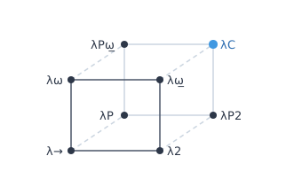
The lambda cube formalizes these distinctions. Starting from the simply typed lambda calculus at the origin, each axis adds a new kind of abstraction:
- x-axis (Polymorphism): Terms can abstract over types. Moving along this axis gives you generic functions like
id : ∀ α, α → αthat work uniformly across all types. - y-axis (Type Operators): Types can abstract over types. This axis adds type-level functions like
ListorMap kthat take types as arguments and produce new types. - z-axis (Dependent Types): Types can depend on terms. Moving along this axis allows types like
Vector α nwhere the type itself contains a value.
The eight vertices represent all possible combinations of these three features:
- λ→ (STLC): The simply typed lambda calculus, with only term-to-term functions. (C, Pascal)
- λ2 (System F): Adds polymorphism, where terms can abstract over types. (Haskell core, ML)
- λω̲: Adds type operators, where types can abstract over types. (Rarely implemented alone)
- λP (LF): Adds dependent types, where types can depend on terms. (Twelf, LF)
- λω (System Fω): Combines polymorphism and type operators. (Haskell with type families, OCaml modules)
- λP2: Combines polymorphism and dependent types. (Rare in practice)
- λPω̲: Combines dependent types and type operators. (Rare in practice)
- λC (CoC): The Calculus of Constructions, combining all three axes. (Lean, Coq, Agda)
Lean sits at λC, the corner where all three meet.
Types as First-Class Citizens
In simple type systems, types and values live in separate worlds. You cannot write a function that takes a type as an argument or returns a type as a result. The wall between them is absolute.
Dependent types tear down this wall. Types become values. You can compute with them, pass them to functions, store them in data structures. The function that constructs Vector Int n takes a number n and returns a type. This uniformity is what makes the whole system work: if types can depend on values, then types must be values.
The theoretical foundations trace through the 20th century: Church’s simply typed lambda calculus, Martin-Löf’s intuitionistic type theory that unified logic and computation, and various attempts to resolve paradoxes that plagued early formal systems. Lean implements a refinement called the Calculus of Inductive Constructions, which adds inductive types and a hierarchy of universes to keep everything consistent. Understanding why that hierarchy exists requires a detour into the history of mathematics.
The practical experience differs from conventional programming. Types become more informative but also more demanding. You must often provide proofs alongside your code, demonstrating that values satisfy required properties. The compiler becomes an adversary that checks your reasoning at every step, as we saw with tactics. When a program type-checks, you gain strong guarantees about its behavior. When it fails, the error messages guide you toward the gap between what you claimed and what you proved.
The Foundational Crisis
This section covers historical background and can be skipped without losing the thread.
By the late 19th century, mathematics faced a crisis of foundations. Mathematicians had built analysis on set theory, set theory on logic, and logic on intuition. The foundations kept shifting. Georg Cantor’s work on infinite sets produced results that seemed paradoxical. The question became urgent: could mathematics be placed on a foundation that was provably secure?
Russell’s Paradox
In 1901, Bertrand Russell sent a letter to Gottlob Frege, who had just completed his life’s work: a logical foundation for all of mathematics. Russell’s letter contained a single question. Consider the set $R$ of all sets that do not contain themselves. Does $R$ contain itself? If yes, then by definition it should not. If no, then by definition it should. Frege’s system was inconsistent. His life’s work collapsed. He wrote back: “Hardly anything more unfortunate can befall a scientific writer than to have one of the foundations of his edifice shaken after the work is finished.”
This is the danger of self-reference. A set that asks about its own membership. A sentence that asserts its own falsehood. A type that contains itself. These constructions look innocent but harbor contradictions. Mathematics needed walls to prevent them.
Hilbert’s Program
David Hilbert proposed an ambitious response. His program, articulated in the 1920s, aimed to formalize all of mathematics in a finite, complete, and consistent axiomatic system. Complete meant every true statement could be proved. Consistent meant no contradiction could be derived. The dream was a mechanical procedure that could, in principle, determine the truth of any mathematical claim. Mathematics would become a closed system, immune to further crisis.
Principia Mathematica, published by Russell and Whitehead between 1910 and 1913, was the most sustained attempt at this vision. Three volumes, nearly 2000 pages, laboriously deriving mathematics from logical axioms. The remark that $1 + 1 = 2$ “will be useful” appears as proposition *54.43 in the first volume, and the arithmetic proof is only completed in the second. The work demonstrated that formalization was possible but also hinted at its costs. The notation was impenetrable, the proofs were tedious, and the system still required axioms whose consistency could not be established from within.
Gödel’s Incompleteness Theorems
Two decades after Principia, Kurt Gödel showed that the consistency problem was not a limitation of Russell’s system but an inescapable feature of mathematics itself. His incompleteness theorems of 1931 proved that any consistent formal system powerful enough to express arithmetic contains true statements that cannot be proved within the system. The first theorem says completeness is impossible: there will always be truths beyond the reach of your axioms. The second theorem is worse: such a system cannot prove its own consistency. The tools Hilbert wanted to use to secure mathematics are necessarily inadequate for the task. You cannot lift yourself by your own bootstraps.
What This Means for Lean
This might seem to doom the entire enterprise of formal verification. If mathematics cannot be complete, if consistency cannot be proved, what is the point of proof assistants?
The answer is that Lean is not attempting Hilbert’s program. Nobody believes Mathlib will eventually contain all mathematical truth or that its foundations can be proved consistent using only its own axioms. The goals are more modest and more practical. What Lean actually provides is mechanical verification of derivations, not philosophical certainty about foundations.
Lean’s kernel accepts a small set of axioms: the rules of the Calculus of Inductive Constructions, plus optional classical principles like the law of excluded middle and the axiom of choice. These axioms are not provably consistent from within the system. They are simply accepted, much as working mathematicians accept ZFC set theory without demanding a consistency proof that Gödel showed cannot exist. Given these axioms, is this proof valid? That question has a definite answer, and Lean provides it.
Yes, there exist true statements about natural numbers that Lean cannot prove. Yes, Lean cannot prove its own consistency. But these limitations do not prevent you from formalizing the theorems mathematicians actually care about. The prime number theorem, the fundamental theorem of calculus, the classification of finite simple groups: none of these bump against incompleteness. The unprovable statements Gödel constructs are specifically engineered to be unprovable. They are curiosities, not obstacles to mathematical practice.
You have not solved Hilbert’s problem. You have sidestepped it. The foundations rest on trust in a small kernel and a handful of axioms that the mathematical community has examined for decades without finding contradiction. The kernel is software, and it has had bugs; soundness holes reachable only through deliberately crafted inputs have been found and fixed over the years, and independent reimplementations such as nanoda and lean4lean exist so that a proof can be re-checked by a second kernel that shares none of the first one’s code. This is not absolute certainty, but it is far more than hand-waving. Principia Mathematica failed because it tried to be a closed system answering every question from first principles. Mathlib succeeds because it tries to be a library: a growing collection of verified results that mathematicians can use, extend, and build upon. The goal is not to end mathematics but to record it in a form that machines can check. That turns out to be achievable, useful, and entirely compatible with Gödel’s theorems.
With the philosophical groundwork laid, we can examine how type theory actually prevents the paradoxes that plagued earlier systems.
Universe Stratification
This section covers advanced material on type universes. Feel free to skim or skip on first reading and return later when universe-related errors arise in practice.
Type theory builds walls against self-reference through stratification. Types are organized into a hierarchy of universes. In Lean, Prop sits at Sort 0, Type 0 sits at Sort 1, Type 1 sits at Sort 2, and so on. A type at level n can only mention types at levels below n. The type Type 0 itself has type Type 1, not Type 0. This breaks the self-reference that doomed Frege’s system. You cannot ask whether Type contains itself because Type is not a single thing; it is an infinite ladder, and each rung can only see the rungs below.
universe u v w

-- Universe polymorphism (explicit universe level)
def polyIdentity (α : Sort u) (a : α) : α := a

-- Universe level expressions
def maxLevel (α : Type u) (β : Type v) : Type (max u v) := α × β

-- Type 0 contains types, Type 1 contains Type 0, etc.
example : Type 0 = Sort 1 := rfl
example : Prop = Sort 0 := rfl

-- Impredicative Prop: functions into Prop stay in Prop
def propPredicate (P : Type u → Prop) : Prop := ∀ α, P α

-- Predicative Type: function types take maximum universe
def typePredicate (P : Type u → Type v) : Type (max (u+1) v) :=
  ∀ α, P α
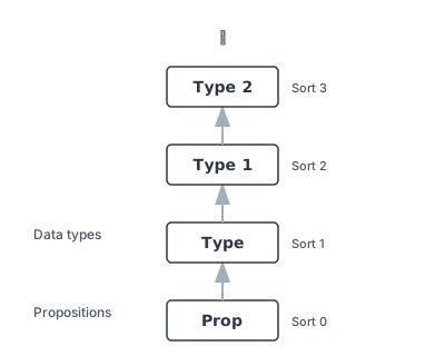
When you write universe u v w in Lean, you are declaring universe level variables. The declaration lets you define functions that work at any universe level. When you write def polyIdentity (α : Sort u) (a : α) : α := a, you are defining a function that works across the entire hierarchy. The Sort u includes both Prop (when u = 0) and Type n (when u = n + 1). This universe polymorphism lets you write single definitions that work everywhere.
The .{u} syntax declares a universe parameter local to a single definition. For file-wide universe variables, use universe u v at the top level:
-- Types themselves have types, forming a hierarchy
#check (Nat : Type 0)      -- Nat lives in Type 0
#check (Type 0 : Type 1)   -- Type 0 lives in Type 1
#check (Type 1 : Type 2)   -- and so on...

-- Universe variables let definitions work at any level
-- The .{u} syntax declares a universe parameter for this definition
def myId.{u} (α : Type u) (x : α) : α := x

-- myId works at any universe level
#check myId Nat 42         -- α = Nat (in Type 0)
#check myId (Type 0) Nat   -- α = Type 0 (in Type 1)
Predicativity
Here is a rule that sounds obvious until you think about it: you cannot be in the photograph you are taking. The photographer stands outside the frame. A committee that selects its own members creates paradoxes of legitimacy. A definition that refers to a collection containing itself is suspect. This intuition, that the definer must stand apart from the defined, is called predicativity.
Imagine a monastery where knowledge is organized into concentric walls. Acolytes in the outer ring may study only texts from their own ring. Scholars who wish to reference the entire outer collection must do so from the second ring, looking inward. Those who would survey the second ring must stand in the third. And so on, each level permitted to see only what lies below. No scholar may cite a collection that includes their own work. The hierarchy prevents the serpent from eating its tail.
This is how predicative universes work. When you quantify over all types at level n, the resulting type lives at level n+1. The definition “for all types α in Type 0, the type α → α” must itself live in Type 1 because it speaks about the entirety of Type 0. You cannot make universal claims about a collection while remaining inside it. The quantification must ascend.
-- Predicative: quantifying over Type u produces Type (u+1)
-- The result must be "larger" than what we quantify over
def predicativeExample : Type 1 := ∀ (α : Type 0), α → α

-- Check the universe levels explicitly
#check (∀ (α : Type 0), α → α : Type 1)  -- Lives in Type 1
#check (∀ (α : Type 1), α → α : Type 2)  -- Lives in Type 2

-- Impredicative: quantifying over Prop still produces Prop
-- Prop can "talk about itself" without ascending universe levels
def impredicativeExample : Prop := ∀ (P : Prop), P → P

#check (∀ (P : Prop), P → P : Prop)  -- Still in Prop, not Type 0!

-- Why this matters: classical logic requires impredicativity
-- "For all propositions P, P or not P" is itself a proposition
def excludedMiddleType : Prop := ∀ (P : Prop), P ∨ ¬P

-- If Prop were predicative, this would be Type 1, breaking classical reasoning
-- Impredicativity lets us define propositions that quantify over all propositions

-- The danger: unrestricted impredicativity leads to paradox
-- Girard's paradox shows Type : Type is inconsistent
-- Lean avoids this by making only Prop impredicative
Lean’s Type hierarchy is predicative: ∀ (α : Type 0), α → α has type Type 1, not Type 0. This prevents Girard’s paradox, a type-theoretic version of Russell’s paradox that arises when Type : Type. The infinite regress of universes is the price of consistency.
Non-Cumulativity
In a cumulative type theory, every type at universe level n is automatically also a type at level n+1 and all higher levels. Coq works this way: if you have Nat : Type 0, you can use Nat anywhere a Type 1 is expected. The type “flows upward” through the hierarchy without explicit intervention. This makes polymorphic code more convenient since you rarely need to think about universe levels.
Lean takes the opposite approach. Each type lives at exactly one universe level. Nat has type Type 0 and only Type 0. If a function expects a Type 1 argument, you cannot pass Nat directly. You must explicitly lift it using ULift or PLift, wrapper types that move values to higher universes.
-- In Lean, Nat has type Type 0, not Type 1
#check (Nat : Type 0)    -- works
-- #check (Nat : Type 1) -- would fail: Nat is not in Type 1

-- A function expecting Type 1 cannot accept Nat directly
def wantsType1 (α : Type 1) : Type 1 := α

-- This fails: Nat lives in Type 0, not Type 1
-- def broken := wantsType1 Nat

-- Solution: explicitly lift Nat to Type 1
def works := wantsType1 (ULift Nat)

-- In a cumulative system (like Coq), this would work:
-- def coqStyle := wantsType1 Nat  -- Coq allows this

-- Practical example: polymorphic container at higher universe
def Container (α : Type 1) := List α

-- Cannot directly use Nat
-- def natContainer := Container Nat  -- fails

-- Must lift first
def natContainer := Container (ULift Nat)

-- Extracting values requires unlifting
def sumLifted (xs : List (ULift Nat)) : Nat :=
  xs.foldl (fun acc x => acc + x.down) 0
Note
This explicit lifting makes universe structure visible in your code. You always know exactly which universe level you are working at. The tradeoff is verbosity: code that would “just work” in Coq requires explicit lifts in Lean. In practice, most Lean code stays within
Type 0andProp, so non-cumulativity rarely causes friction.
The World of Prop
Lean’s universe hierarchy has a special member at the bottom: Prop, the universe of propositions. Unlike Type, which holds computational data, Prop holds logical statements. This distinction enables two features that would be dangerous elsewhere: impredicativity and proof irrelevance. Together, they make Prop a safe space for classical reasoning.
Impredicativity of Prop
Prop breaks the predicativity rule. While ∀ (α : Type 0), α → α must live in Type 1, the analogous ∀ (P : Prop), P → P has type Prop, staying at the same level despite quantifying over all propositions. The monastery has a secret inner sanctum where the old restrictions do not apply.
-- PLift: lifts any type by exactly one level
def liftedFalse : Type := PLift False

-- ULift: lifts types by any amount
def liftedNat : Type u := ULift.{u} Nat

-- Lifting and unlifting values
def liftExample : ULift.{1} Nat := ⟨42⟩
example : liftExample.down = 42 := rfl

-- Non-cumulativity: types exist at exactly one level
def needsLifting (α : Type 1) : Type 2 := ULift.{2} α
This matters for classical logic. The law of excluded middle, ∀ (P : Prop), P ∨ ¬P, quantifies over all propositions. If Prop were predicative, this would live in Type 0, making it a computational object rather than a logical axiom. But how is impredicativity safe here when it causes paradoxes elsewhere?
Proof Irrelevance
The answer is proof irrelevance. A bear catching a salmon does not care whether the fish swam upstream via the left channel or the right. Proof irrelevance applies this principle to mathematics: any two proofs of the same proposition are equal. If you have two proofs p1 and p2 that both establish proposition P, then p1 = p2 holds definitionally. We care that the theorem is true, not which path led there.
-- Basic logical connectives
theorem and_intro (P Q : Prop) (hp : P) (hq : Q) : P ∧ Q := ⟨hp, hq⟩

theorem or_elim (P Q R : Prop) (h : P ∨ Q) (hp : P → R) (hq : Q → R) : R :=
  h.elim hp hq

theorem iff_intro (P Q : Prop) (hpq : P → Q) (hqp : Q → P) : P ↔ Q :=
  ⟨hpq, hqp⟩

-- Proof irrelevance demonstration
theorem proof_irrel_demo (P : Prop) (p1 p2 : P) : p1 = p2 := rfl

-- Classical logic (via choice)
open Classical in
theorem excluded_middle (P : Prop) : P ∨ ¬P := Classical.em P
The technical foundation is that Prop is a subsingleton universe. A subsingleton is a type with at most one element. For any proposition P, there is at most one proof of P up to definitional equality. This contrasts with Type, where Bool has two distinct elements true and false, and Nat has infinitely many.
What makes impredicativity safe is that Prop is computationally inert. You cannot eliminate a proof into Type to build data from it (except for subsingletons, where the result is forced), so an impredicative definition over propositions can never be used to construct the kind of self-referential data that produces paradoxes. Proof irrelevance is the companion to this restriction: if proofs cannot be told apart, there is nothing to extract from them anyway. The serpent may eat its tail here because the tail has no substance.
Computational Erasure
Proof irrelevance has profound computational implications. Because all proofs of a proposition are equal, the compiler can erase proofs at runtime. A function that takes a proof argument does not actually need to receive any runtime data for that argument. This erasure is essential for performance: without it, complex proofs would bloat compiled code with useless proof terms. Your elaborate justification for why the code is correct compiles down to nothing, much like comments but with mathematical guarantees.
Proof irrelevance also enables powerful automation. When a tactic constructs a proof term, the exact structure of that term does not matter. The tactic can use whatever construction is convenient, and the result will be equal to any other proof of the same statement. This freedom simplifies tactic implementation and allows for aggressive optimization of proof search.
Constructive and Classical Logic
Constructive logic gives proofs a computational interpretation, but Lean distinguishes logical existence from data you can execute. A proof of ∃ n : Nat, P n lives in Prop: you may use its witness while proving another proposition, but cannot in general pattern-match on it to return a Nat. To return an executable witness together with its property, use a subtype such as {n : Nat // P n}, as below. Sigma types package a witness with a component in Type; Σ n : Nat, P n is not well-typed when P n : Prop. Classical choice can select a witness from an existential proof, but that selection is noncomputable.
-- Constructive proof: we provide an explicit witness
theorem constructive_exists : ∃ n : Nat, n * n = 4 :=
  ⟨2, rfl⟩  -- The witness is 2, and we can compute 2 * 2 = 4

-- Constructive: we can extract and run the witness
def constructive_even : { n : Nat // n % 2 = 0 } :=
  ⟨4, rfl⟩  -- The subtype bundles value with proof

#eval constructive_even.val  -- Outputs: 4

-- The law of excluded middle itself (classical axiom)
theorem lem (P : Prop) : P ∨ ¬P := Classical.em P

-- Double negation elimination (classical, not constructive)
-- In constructive logic, ¬¬P does not imply P
theorem dne (P : Prop) : ¬¬P → P := Classical.byContradiction

-- Classical proof by contradiction: no even number is odd
theorem even_not_odd (n : Nat) : n % 2 = 0 → ¬(n % 2 = 1) := by
  intro heven hodd
  omega
Classical logic adds axioms that break this computational interpretation. The law of excluded middle (P ∨ ¬P for any proposition) lets you prove existence by contradiction without producing a witness. Double negation elimination (¬¬P → P) lets you escape a double negation without constructing a direct proof. These principles are mathematically sound but computationally empty. A classical existence proof need not provide an executable witness.
Lean provides classical axioms through the Classical namespace. When you use Classical.em or tactics like by_contra, you are stepping outside constructive logic. Lean tracks this: a definition whose computation depends on an axiom (or on another noncomputable definition) must be marked noncomputable, meaning it cannot be evaluated at runtime. Classical reasoning inside proofs and types does not count, since proofs are erased before the program runs; only the data the definition actually produces matters.
-- Classical choice: given existence, extract a witness
-- This is noncomputable because we cannot run it
noncomputable def classical_witness (P : Nat → Prop) (h : ∃ n, P n) : Nat :=
  Classical.choose h

-- The witness satisfies the property (but we cannot compute what it is)
theorem classical_witness_spec (P : Nat → Prop) (h : ∃ n, P n) :
    P (classical_witness P h) :=
  Classical.choose_spec h

-- Contrast: decidable existence gives computable witnesses
def decidable_witness (p : Nat → Bool) (bound : Nat) : Nat :=
  -- We can search by enumeration because the domain is finite
  (List.range bound).find? (fun n => p n) |>.getD 0

-- The key insight: constructive proofs compute, classical proofs assert
Why does this matter? An executable sorting function can carry a proof that its result is sorted, and that proof may use classical reasoning because proofs are erased. Merely proving ∃ ys, Sorted ys ∧ ... does not give an executable sorting function, even if the existence proof is constructive: the result is still in Prop. The distinction is between the data a definition returns and the logical evidence accompanying it.
The practical guidance: use constructive methods when you can, classical when you must. Lean supports both. The noncomputable modifier tells Lean not to generate executable code for a definition; a common reason is that its result depends on Classical.choice. When a definition lacks that marker, the compiler can run it, even if the proofs attached to it reason classically. The type system tracks the distinction so you always know which world you are in.
Type Equivalences
When are two types “the same”? Having functions in both directions is not enough. You can map Bool to Nat and back, but Nat has infinitely many values while Bool has two. The round-trip loses information.
An equivalence \(A \simeq B\) requires functions in both directions that are mutual inverses: composing them in either order gives back the original value. This captures the idea that \(A\) and \(B\) have the same structure, just with different names for their elements.
-- Two types are "the same" when they are equivalent
-- An equivalence requires functions in both directions that are mutual inverses

variable {α β γ : Type*}

-- Having functions both ways is NOT enough
def boolToNat : Bool → Nat
  | true => 1
  | false => 0

def natToBool : Nat → Bool
  | 0 => false
  | _ => true

-- These are NOT inverses: natToBool (boolToNat true) = true, but
-- boolToNat (natToBool 42) = 1, and natToBool 1 = true ≠ 42

-- A proper equivalence between Unit ⊕ Unit and Bool
-- Both have exactly two elements
def sumUnitEquivBool : Unit ⊕ Unit ≃ Bool where
  toFun | .inl () => false | .inr () => true
  invFun | false => .inl () | true => .inr ()
  left_inv := by intro x; cases x <;> rfl
  right_inv := by intro b; cases b <;> rfl

-- Equivalences compose
example : (α ≃ β) → (β ≃ γ) → (α ≃ γ) := Equiv.trans

-- Equivalences are symmetric
example : (α ≃ β) → (β ≃ α) := Equiv.symm

-- Every type is equivalent to itself
example : α ≃ α := Equiv.refl α

-- Product types commute (up to equivalence)
def prodComm : α × β ≃ β × α where
  toFun p := (p.2, p.1)
  invFun p := (p.2, p.1)
  left_inv := by intro ⟨a, b⟩; rfl
  right_inv := by intro ⟨b, a⟩; rfl

-- Currying is an equivalence
def curryEquiv : (α × β → γ) ≃ (α → β → γ) where
  toFun f a b := f (a, b)
  invFun g p := g p.1 p.2
  left_inv := by intro f; ext ⟨a, b⟩; rfl
  right_inv := by intro g; rfl
Equivalences form a well-behaved notion of sameness. They are reflexive (every type is equivalent to itself), symmetric (if \(A \simeq B\) then \(B \simeq A\)), and transitive (equivalences compose). This makes them an equivalence relation on types, which is exactly what you want for a notion of “sameness.”
The distinction matters in mathematics and programming alike. When you prove that two types are equivalent, you can transport theorems and constructions between them. If you prove a property about Bool, the equivalence \(\text{Unit} \oplus \text{Unit} \simeq \text{Bool}\) lets you conclude the same property holds for the sum type. Mathlib uses equivalences extensively to connect different representations of the same mathematical structure.
Quotients and Parametricity
Quotient types allow you to define new types by identifying elements of an existing type according to an equivalence relation. The integers modulo n, for example, identify natural numbers that have the same remainder when divided by n. Quotients are essential for constructing mathematical objects like rational numbers, real numbers, and algebraic structures.
-- Simple modulo equivalence relation
def ModRel (n : Nat) : Nat → Nat → Prop :=
  fun a b => a % n = b % n

-- Prove it's an equivalence relation
theorem ModRel.refl (n : Nat) : ∀ x, ModRel n x x :=
  fun _ => rfl

theorem ModRel_symm (n : Nat) : ∀ x y, ModRel n x y → ModRel n y x :=
  fun _ _ h => h.symm

theorem ModRel.trans (n : Nat) : ∀ x y z, ModRel n x y → ModRel n y z → ModRel n x z :=
  fun _ _ _ hxy hyz => Eq.trans hxy hyz

-- Create a setoid for a given modulus
def ModSetoid (n : Nat) : Setoid Nat where
  r := ModRel n
  iseqv := {
    refl := ModRel.refl n
    symm := @ModRel_symm n
    trans := @ModRel.trans n
  }

-- Define the quotient type (integers modulo n)
def ZMod (n : Nat) : Type := Quotient (ModSetoid n)
Quotients come with a well-definedness obligation that ordinary types do not have, and the way Lean discharges it has a cost: Quot.sound is an axiom, and the computation rule for Quot.lift is a primitive the kernel must implement rather than something derived from an inductive type. The usual meta-theoretic argument for parametricity, the principle that a function of type ∀ α, α → α must be the identity because it has no way to inspect α, does not extend to the quotient primitives for free.
The proof obligation on Quot.lift is the user-facing half of this. When you lift a function to operate on a quotient type, you must prove that the function respects the equivalence relation. Without that proof, a function could distinguish two representatives of the same equivalence class, and the quotient would stop being a quotient.
namespace ZMod

-- Constructor respecting equivalence
def mk (n : Nat) (a : Nat) : ZMod n :=
  Quotient.mk (ModSetoid n) a

-- Addition operation via lifting
def add {n : Nat} [NeZero n] : ZMod n → ZMod n → ZMod n :=
  Quotient.lift₂
    (fun a b => mk n ((a + b) % n))
    (fun a₁ a₂ b₁ b₂ h₁ h₂ => by
      apply Quotient.sound
      simp +instances only [ModSetoid] at h₁ h₂ ⊢
      unfold ModRel at h₁ h₂ ⊢
      rw [Nat.add_mod, h₁, h₂, ← Nat.add_mod]
      rfl)

-- Quotient.sound: related elements are equal
theorem mk_eq_of_rel {n : Nat} (a b : Nat) (h : ModRel n a b) :
  mk n a = mk n b :=
  Quotient.sound h

-- Quotient induction principle
theorem ind_on {n : Nat} {P : ZMod n → Prop} (q : ZMod n)
  (h : ∀ a, P (mk n a)) : P q :=
  Quotient.ind h q

end ZMod
Why is this acceptable? Quotients are a convenient foundation for many mathematical constructions, including equivalence classes of Cauchy sequences. They are not the only way to represent numbers: Lean’s Int uses constructors for nonnegative and negative integers, and Rat uses a normalized fraction representation. The extra trusted surface is confined to the quotient primitives. Requiring lifted functions to respect equivalence ensures that quotient operations cannot distinguish equivalent representatives.
Comparative Type Systems
Different languages make different design choices in their type systems. The following table summarizes key features across proof assistants and programming languages.
| Feature | Lean 4 | Coq | Agda | Idris 2 | Haskell | Rust |
|---|---|---|---|---|---|---|
| Dependent Types | Full | Full | Full | Full | Limited | No |
| Universe Hierarchy | Predicative | Predicative | Predicative | Type : Type | None | None |
| Universe Cumulativity | No | Yes | No | N/A | N/A | N/A |
| Proof Irrelevance | Yes (Prop) | Yes (SProp; not ordinary Prop) | Optional | Erasure | N/A | N/A |
| Tactic Language | Lean DSL | Ltac | No | Elab | N/A | N/A |
| Type Inference | Partial | Partial | Partial | Partial | Full* | Full |
| Termination Checking | Required | Required | Required | Optional | No | No |
| Linear Types | No | No | No | QTT | Extension | Ownership |
| Effects System | Monad | Monad | Monad | Algebraic | Monad | Ownership |
| Code Generation | Native | OCaml/Haskell | Haskell | Native | Native | Native |
| Cubical Type Theory | No | No | Yes | No | No | No |
Glossary:
- Ltac: Coq’s original tactic language, a dynamically-typed scripting language for proof automation
- QTT: Quantitative Type Theory, tracks how many times each variable is used to enable linear resource management
- Erasure: Idris 2 has no proof-irrelevant universe; QTT erases values of quantity 0 at runtime, which gives a similar effect
- Type : Type: Idris 2 has a single universe that contains itself, trading consistency as a logic for simplicity
- Predicative: A universe is predicative if quantifying over types at level n produces a type at level n+1 or higher
- Cumulativity: Whether a type at level n is automatically also at level n+1
- *: Haskell 2010 has full type inference, but enabling extensions (GADTs, TypeFamilies, RankNTypes, UndecidableInstances) may require type annotations or introduce undecidability
Lean and Coq provide full dependent types with rich proof automation, making them suitable for formal verification. Agda emphasizes explicit proof terms and supports cubical type theory for constructive equality, connecting to homotopy type theory and higher topos theory. Idris 2 uses quantitative type theory to track resource usage, bridging the gap between theorem proving and systems programming.
Haskell approaches dependent types through extensions like GADTs, DataKinds, and type families. Base Haskell maintains decidable type checking, but common extensions can introduce undecidability. The language proved enormously influential as a research vehicle, demonstrating what expressive type systems could achieve. However, approximating dependent types through dozens of extensions bolted onto a core calculus not designed for them creates inherent complexity. Type-level programming in Haskell requires navigating interactions between GADTs, type families, DataKinds, and numerous other extensions, each with its own quirks and limitations. For projects that need the full expressive power of dependent types, languages built on richer type theories from first principles offer a cleaner foundation.
Rust’s ownership system provides memory safety guarantees through affine types, with decidable checking and predictable compile times. However, Rust’s type system proves memory safety, not functional correctness. The borrow checker ensures you will not have use-after-free bugs, but it cannot verify that your sorting algorithm actually sorts or that your cryptographic protocol maintains confidentiality. Proving Rust code correct requires external tools like Prusti, Creusot, Kani, or Verus. These tools have achieved real successes verifying cryptographic primitives and isolated algorithms, but verifying the business logic of production systems remains an active research frontier. CompCert addresses a different problem: it compiles C to assembly with a semantic preservation proof. Its compiler implementation is extracted from Coq to OCaml; it does not extract verified C programs from high-level specifications. A verified translation from a Lean program to Rust would require a separate correctness argument. Even without extraction, useful techniques remain: differential testing between a proven specification and a Rust implementation, or model-based testing over an explicitly bounded domain. These approaches yield a spectrum of assurance, from probabilistic confidence through exhaustive bounded testing to machine-checked proofs about the model. A fully verified pipeline to production Rust remains hard, but partial verification still delivers industrial value. The Rust Formal Methods Interest Group coordinates ongoing work.
A common critique of Lean is its lack of linear or affine types, which would enable compile-time guarantees about resource usage and in-place mutation. This is a deliberate architectural choice, not an oversight. Rust verifies resource management statically at compile time through ownership; Lean minimizes the performance cost of immutability dynamically at runtime through FBIP (functional but in-place) optimizations and reference counting. The trade-off: Lean’s simpler type system makes large-scale theorem proving more tractable, since proofs do not need to thread linearity constraints through every function. You can share data freely without borrow checker complexity, and FBIP recovers imperative performance for the common case where data has a single owner.
The table above looks like a feature comparison. It is actually a map of philosophical commitments. Each row is a question about the nature of computation; each column is an answer. The language you choose chooses what thoughts are easy to think.
The fundamental trade-off is expressiveness versus automation. Full dependent types let you express arbitrary properties but require manual proof effort. Decidable type systems like Rust and Haskell infer types automatically but cannot express many important invariants. Choose based on whether you need machine-checked proofs or just strong static guarantees.
In short: Lean and Coq make you prove everything is correct, Rust makes you prove memory is safe, Haskell makes you prove effects are tracked, and most other languages just trust you not to ship on Friday.
Compiler Options
The set_option command configures compiler behavior. Most options control elaboration and pretty-printing. You will rarely need these until you hit edge cases:
-- set_option configures compiler and elaborator behavior
-- Show implicit arguments that are normally hidden
set_option pp.explicit true in
#check @id Nat 5  -- shows: @id Nat 5 : Nat

-- maxRecDepth controls recursion during elaboration and kernel checking,
-- not runtime. #reduce fully unfolds expressions at compile time:
-- #reduce (List.range 500).length  -- ERROR without increased limit
set_option maxRecDepth 4000 in
#reduce (List.range 500).length  -- 500
The @ prefix forces explicit argument mode: @id Nat 5 passes the type Nat explicitly instead of letting Lean infer it. Combined with set_option pp.explicit true, this shows all normally-hidden arguments. The maxRecDepth option increases how deeply Lean will recurse during elaboration. The same limit also bounds the kernel’s type checker, so a “deep recursion detected” error behaves the same on every machine rather than depending on the native stack size.
Where Types Meet Values
Type theory provides the foundation. The next article explores dependent types in depth: how types can depend on values, how propositions become types, and how proofs become programs. This is where Lean’s power as a theorem prover emerges from its foundations as a programming language.